International Finance

Options Primer: Pricing and Payoffs

Main issues

• What is an option? Calls, puts, and the four basic positions

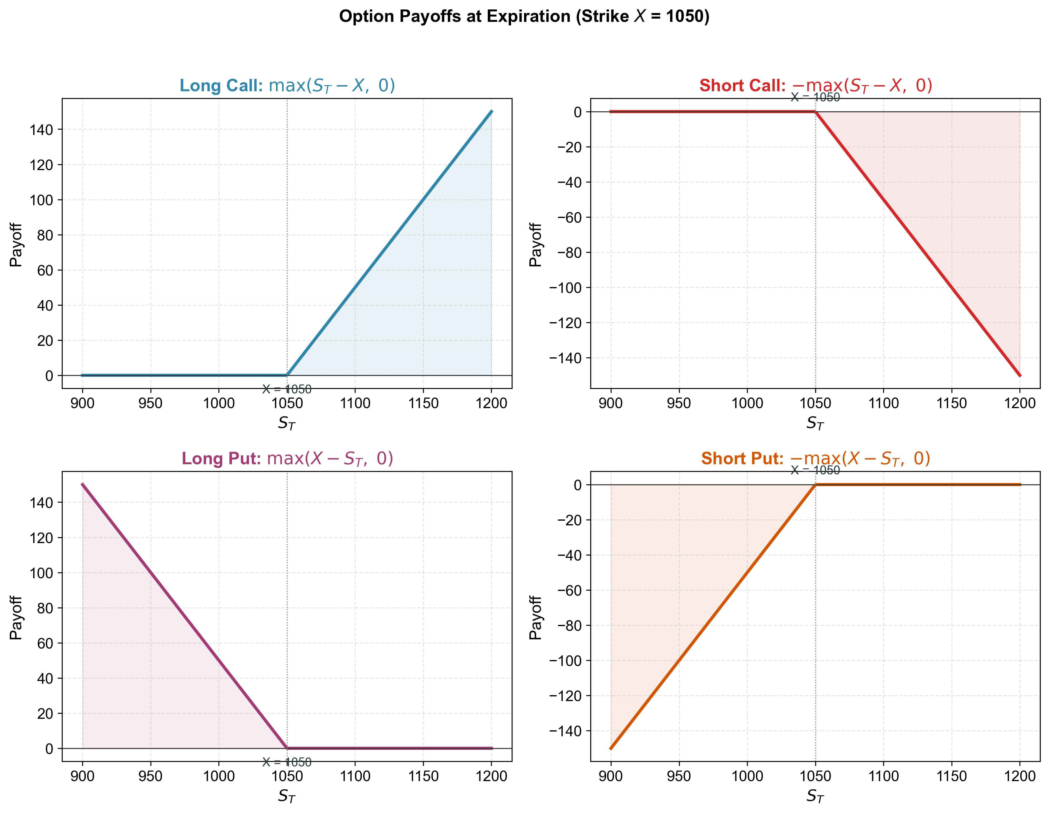
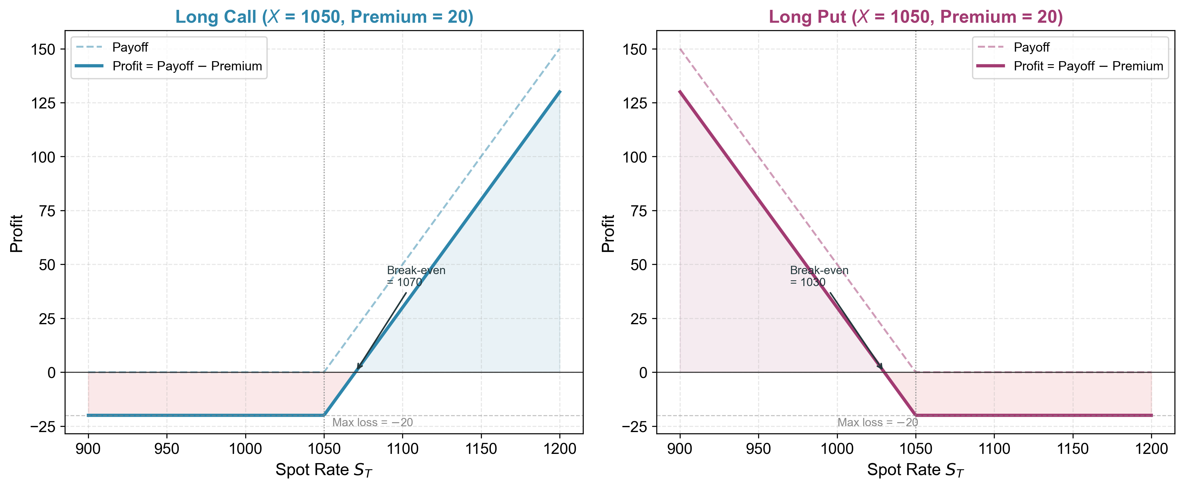
• Payoff diagrams: visualizing option positions at expiration

• FX options: conventions, intrinsic value, and key price drivers

• Put-call parity: the fundamental link between calls, puts, and forwards

• Binomial option pricing: one period, multi-period, and convergence to Garman-Kohlhagen

This primer provides the pricing background used in Lecture 8 (Nonlinear Exposure and FX Options).

This is a technical primer. Lecture 8 focuses on why firms need options and how to use them strategically. This primer covers the mechanics: what options are, how their payoffs work, and how they are priced using no-arbitrage arguments.

What Is an Option?

Definition

An option gives the holder the right, but not the obligation, to buy or sell an asset at a predetermined price.

• Call option: right to buy the underlying at the strike price \(X\)

• Put option: right to sell the underlying at the strike price \(X\)

Key distinction from forwards:

• A forward obligates both parties. An option gives a choice.

• This asymmetry has value — the buyer pays a premium upfront.

Long vs. short positions

	Long (buyer)	Short (seller/writer)
Pays	Premium upfront	—
Receives	Right to exercise	Premium upfront
Risk	Limited to premium	Potentially unlimited
Motivation	Insurance / speculation	Earn premium income

• The buyer pays for optionality — the right to walk away if the option is not favorable

• The seller is obligated to deliver if the buyer exercises

• Zero-sum game: buyer’s gain = seller’s loss

European vs. American

• European option: can only be exercised at expiration

• American option: can be exercised at any time before expiration

In foreign exchange markets:

• Most traded FX options are European style

• Simplifies pricing: only need to consider the terminal payoff

• American options are more complex (early exercise premium) but rare in FX

Throughout this primer, all options are European.

Payoff Diagrams

The four basic positions

Long call: \(\max(S_T - X,\; 0)\)

• Profits when \(S_T > X\); loss capped at zero payoff

Short call: \(-\max(S_T - X,\; 0)\)

• Mirror image of long call; seller’s obligation

Long put: \(\max(X - S_T,\; 0)\)

• Profits when \(S_T < X\); loss capped at zero payoff

Short put: \(-\max(X - S_T,\; 0)\)

• Mirror image of long put; seller’s obligation

Payoff diagrams

Four panels showing the payoff (not profit) of each position. Notice the kinks at the strike price X. The buyer’s positions have a floor at zero; the seller’s positions have a ceiling at zero. Payoff is not the same as profit — we haven’t subtracted the premium yet.

From payoff to profit

Profit = Payoff \(-\) Premium

• The buyer pays the premium upfront, so profit shifts the payoff curve down by the premium amount

• Break-even for a long call: \(S_T = X + \text{Premium}\)

• Break-even for a long put: \(S_T = X - \text{Premium}\)

• Maximum loss for the buyer: the premium paid (limited downside)

• Maximum loss for the seller: potentially unlimited (call) or up to \(X\) (put)

Profit diagrams

The dashed lines show payoff, the solid lines show profit (payoff minus premium). Notice how the break-even points shift away from the strike by the premium amount. The shaded regions show where each position makes or loses money.

FX Options

FX option = right to exchange currencies

An FX option gives the right to exchange one currency for another at a fixed rate.

• A “EUR call / USD put” is the right to buy EUR and sell USD at strike \(X\) (USD/EUR)

• A “EUR put / USD call” is the right to sell EUR and buy USD at strike \(X\)

Convention: An FX option is simultaneously a call on one currency and a put on the other.

Example: A EUR call with \(X = 1.10\) USD/EUR gives the right to buy EUR 1 for USD 1.10.

• Exercise if \(S_T > 1.10\): buy EUR cheaply at 1.10 and sell at market rate \(S_T\)
• Don’t exercise if \(S_T < 1.10\): buy EUR at the cheaper market rate instead

The forward rate as the center

Recall from Lecture 4 (Covered Interest Parity):

\[F = S_0 \times \frac{1 + r}{1 + r^*}\]

• The forward rate \(F\) is the “center” of option pricing

• At-the-money forward (ATMF): strike \(X = F\) — call and put have equal value

• In-the-money (ITM): call with \(X < F\), or put with \(X > F\)

• Out-of-the-money (OTM): call with \(X > F\), or put with \(X < F\)

Intrinsic value = value if exercised immediately against the forward:

• Call: \(\max(F - X,\; 0)\)

• Put: \(\max(X - F,\; 0)\)

Time value = Option price \(-\) Intrinsic value (always \(\geq 0\))

Factors affecting option prices

Five key inputs determine option value:

Factor	Call price	Put price	Intuition
Forward \(F\) \(\uparrow\)	\(\uparrow\)	\(\downarrow\)	Higher expected terminal rate
Strike \(X\) \(\uparrow\)	\(\downarrow\)	\(\uparrow\)	Harder/easier to exercise
Volatility \(\sigma\) \(\uparrow\)	\(\uparrow\)	\(\uparrow\)	More chance of large moves
Time to expiry \(T\) \(\uparrow\)	\(\uparrow\)	\(\uparrow\)	More time for favorable moves
Interest rate \(r\) \(\uparrow\)	\(\uparrow\)	\(\downarrow\)	Discounting + forward effect

Volatility is the most important input — it measures how much the exchange rate might move. Higher volatility \(\Rightarrow\) more “upside” for the option buyer \(\Rightarrow\) higher price.

Put-Call Parity

The fundamental link

For European options with the same strike and expiry:

\[\boxed{c - p = \frac{F - X}{1 + r}}\]

where \(c\) = call price, \(p\) = put price, \(F\) = forward rate, \(X\) = strike, \(r\) = domestic interest rate.

This is a no-arbitrage relationship, not a model — it holds regardless of what pricing model you use.

Put-call parity links calls, puts, and forwards. It is model-free because it relies only on the absence of arbitrage. If it were violated, you could construct a riskless profit by trading the three instruments.

Proof by replication

Consider two portfolios at time 0:

Portfolio A: Long call + invest \(\frac{X}{1+r}\) in domestic bonds

Portfolio B: Long put + long forward at rate \(F\) + invest \(\frac{F}{1+r}\) in domestic bonds

At expiration \(T\):

State	Portfolio A	Portfolio B
\(S_T > X\)	\((S_T - X) + X = S_T\)	\(0 + (S_T - F) + F = S_T\)
\(S_T \leq X\)	\(0 + X = X\)	\((X - S_T) + (S_T - F) + F = X\)

Both give \(\max(S_T, X)\) at \(T\). Same payoff \(\Rightarrow\) same price today:

\[c + \frac{X}{1+r} = p + 0 + \frac{F}{1+r} \quad \Rightarrow \quad c - p = \frac{F - X}{1+r}\]

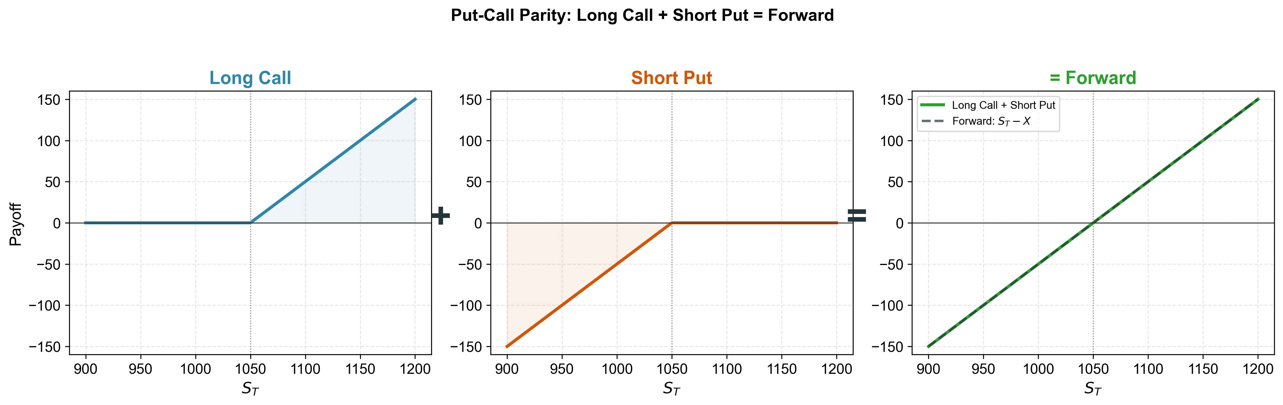
Visual: long call + short put = forward

Key implication: A forward is just a combination of a call and a put at the same strike.

At strike \(X = F\): the call and put have equal value (\(c = p\)).

Numerical example

Setup: \(S_0 = 1000\), \(r = 5\%\), \(r^* = 4\%\), \(X = 1050\)

Forward rate: \(F = 1000 \times \frac{1.05}{1.04} \approx 1009.6\)

Put-call parity: \(c - p = \frac{F - X}{1 + r} = \frac{1009.6 - 1050}{1.05} = \frac{-40.4}{1.05} = -38.5\)

So \(c = p - 38.5\). The call is cheaper than the put because the strike is above the forward.

• If someone quotes you \(p = 60\), then \(c = 60 - 38.5 = 21.5\)

• If you know the call price, you get the put price for free (and vice versa)

One-Period Binomial Model

Setup

Two possible states at \(T\): the exchange rate goes up to \(S_u\) or down to \(S_d\).

The call has known payoffs: \(c_u = \max(S_u - X, 0)\) and \(c_d = \max(S_d - X, 0)\).

Question: What is the fair price \(c_0\) today?

The replication idea

Key insight: We can replicate the option payoff using two instruments:

1. \(\Delta\) units of a forward contract (costs nothing to enter)

2. \(B\) dollars invested in a domestic bond (earns \(r\))

Replicating portfolio payoffs at \(T\):

• Up state: \(\Delta(S_u - F) + B(1 + r) = c_u\)

• Down state: \(\Delta(S_d - F) + B(1 + r) = c_d\)

Two equations, two unknowns. Solve for \(\Delta\) and \(B\).

Solving for the option price

Subtract down from up:

\[\Delta(S_u - S_d) = c_u - c_d \quad \Rightarrow \quad \boxed{\Delta = \frac{c_u - c_d}{S_u - S_d}}\]

\(\Delta\) is the hedge ratio — how many forwards replicate the option.

From the down-state equation:

\[B = \frac{c_d - \Delta(S_d - F)}{1 + r}\]

Option price = cost of replicating portfolio = \(B\) (forward is free to enter)

\[\boxed{c_0 = B = \frac{c_d - \Delta(S_d - F)}{1 + r}}\]

No probabilities needed!

Notice: we never used the probability of up vs. down.

• The option price comes purely from no-arbitrage — if the option is mispriced relative to \(B\), there is a riskless profit

• Different investors can disagree about probabilities and still agree on the price

• This is the power of replication: price by matching payoffs, not by forecasting

This is the same logic behind CIP (Lecture 4) and forward pricing:

• If two strategies have the same payoff, they must have the same price

• Otherwise: arbitrage

Risk-neutral pricing

An equivalent and often more convenient approach. Define:

\[\boxed{q = \frac{F - S_d}{S_u - S_d}}\]

Then the option price can be written as:

\[c_0 = \frac{q \cdot c_u + (1 - q) \cdot c_d}{1 + r}\]

• \(q\) is the risk-neutral probability — it makes the expected rate equal to the forward

• Not a real-world probability — it’s the probability that is consistent with no-arbitrage pricing

• Equivalent to the replication approach, but often faster to compute

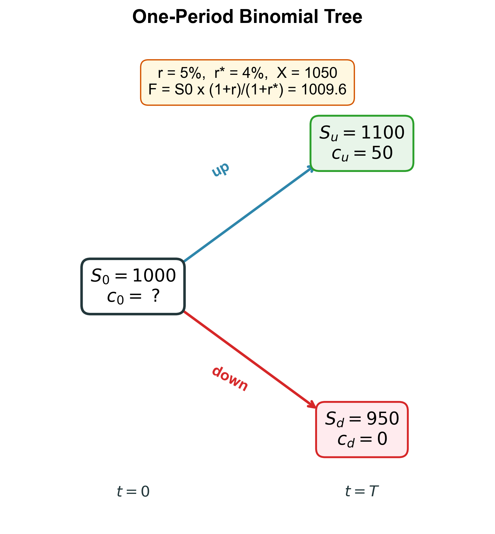
Numerical example

Setup: \(S_0 = 1000\), \(S_u = 1100\), \(S_d = 950\), \(r = 5\%\), \(r^* = 4\%\), \(X = 1050\)

\(F = 1000 \times \frac{1.05}{1.04} \approx 1009.6\), \(\quad c_u = 50\), \(\quad c_d = 0\)

Delta: \(\Delta = \frac{50 - 0}{1100 - 950} = \frac{50}{150} = \frac{1}{3}\)

Bond: \(B = \frac{0 - \frac{1}{3}(950 - 1009.6)}{1.05} = \frac{0 + 19.87}{1.05} = 18.92\)

Option price: \(c_0 = B = 18.92\)

Check with risk-neutral pricing:

\(q = \frac{1009.6 - 950}{1100 - 950} = \frac{59.6}{150} = 0.397\)

\(c_0 = \frac{0.397 \times 50 + 0.603 \times 0}{1.05} = \frac{19.87}{1.05} = 18.92\) \(\checkmark\)

Multi-Period Binomial Model

From one period to two

The tree recombines: an up move followed by a down move gives the same node as down-then-up. This is critical for computational efficiency — with N periods, we have N+1 terminal nodes instead of 2^N.

Working backwards

Backward induction: Start from the terminal payoffs and work backwards one period at a time.

At each node, apply the one-period formula with the same risk-neutral probability:

\[q = \frac{f_{\Delta t} - d}{u - d} \qquad \text{where } f_{\Delta t} = \frac{1 + r_{\Delta t}}{1 + r^*_{\Delta t}}\]

Step 1: Terminal payoffs — \(c = \max(S_T - X, 0)\) at each final node

Step 2: At each period-1 node: \(c = \frac{q \cdot c_u + (1-q) \cdot c_d}{1 + r_{\Delta t}}\)

Step 3: At the root: same formula using the period-1 values

Each backward step is just the one-period model applied locally.

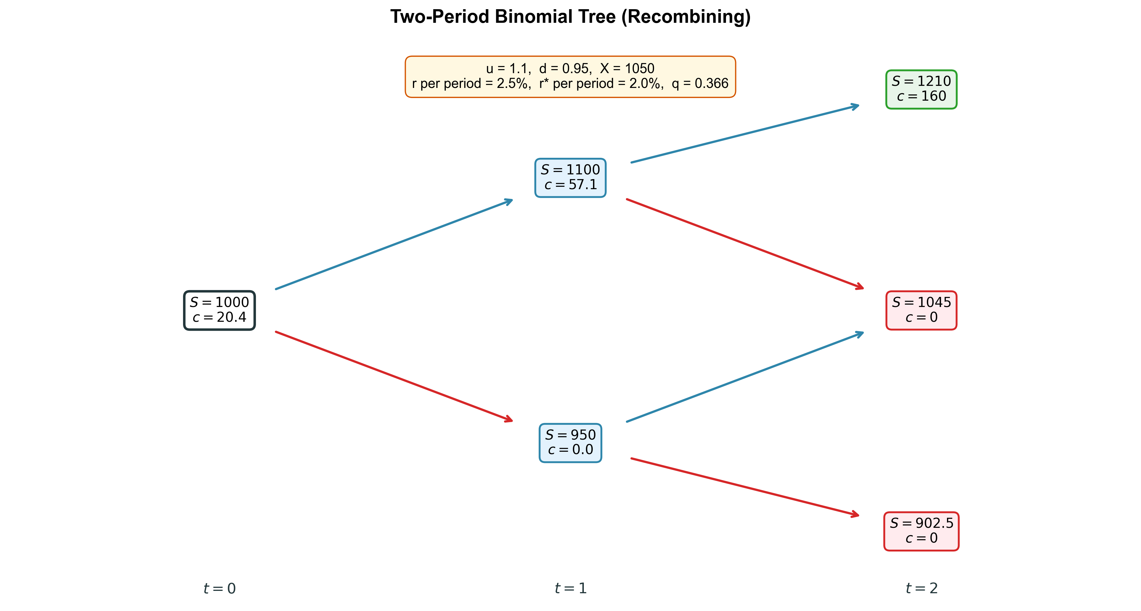
Two-period example

Using \(u = 1.10\), \(d = 0.95\), \(X = 1050\), \(r_{\Delta t} = 2.5\%\), \(r^*_{\Delta t} = 2.0\%\):

Terminal payoffs:

• \(S_{uu} = 1210\): \(c_{uu} = \max(1210 - 1050, 0) = 160\)

• \(S_{ud} = 1045\): \(c_{ud} = \max(1045 - 1050, 0) = 0\)

• \(S_{dd} = 902.5\): \(c_{dd} = 0\)

Risk-neutral probability: \(q = \frac{1.025/1.02 - 0.95}{1.10 - 0.95} = \frac{0.0549}{0.15} = 0.366\)

Period 1 (up node): \(c_u = \frac{0.366 \times 160 + 0.634 \times 0}{1.025} = \frac{58.6}{1.025} = 57.1\)

Period 1 (down node): \(c_d = \frac{0.366 \times 0 + 0.634 \times 0}{1.025} = 0\)

Period 0: \(c_0 = \frac{0.366 \times 57.1 + 0.634 \times 0}{1.025} = \frac{20.9}{1.025} = 20.4\)

From 2 to N periods

The two-period model extends naturally:

• Split the time horizon \(T\) into \(N\) equal periods of length \(\Delta t = T/N\)

• Each period has up factor \(u\) and down factor \(d\)

• Tree has \(N+1\) terminal nodes (recombining), backward induction from the end

Key question: How to choose \(u\) and \(d\)?

Cox-Ross-Rubinstein (CRR) calibration:

\[\boxed{u = e^{\sigma\sqrt{\Delta t}}, \qquad d = \frac{1}{u} = e^{-\sigma\sqrt{\Delta t}}}\]

• \(\sigma\) = annualized volatility of the exchange rate

• As \(N\) increases, \(\Delta t \to 0\) and the binomial model produces finer and finer approximations

• The tree structure ensures \(d = 1/u\) so the tree recombines

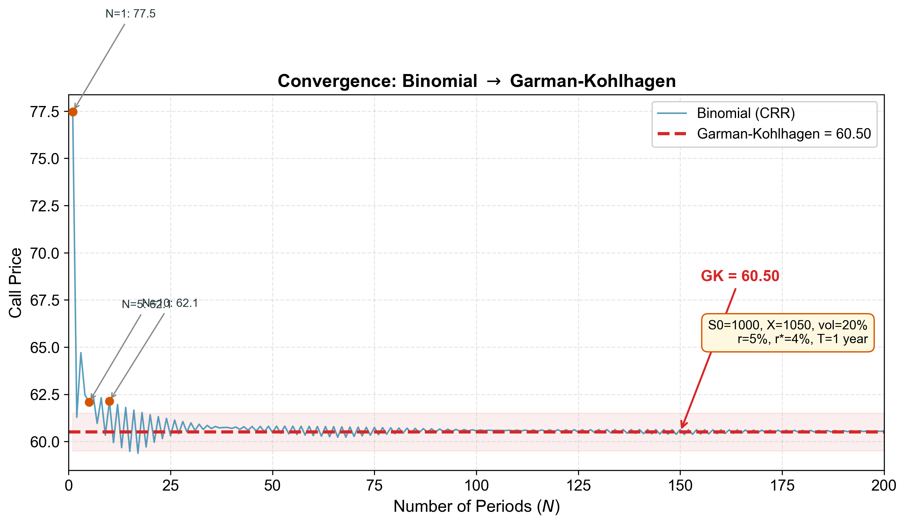
Convergence to Black-Scholes

Binomial \(\to\) Garman-Kohlhagen

The oscillating blue line is the binomial price as a function of the number of periods N. It converges rapidly to the GK price (red dashed line). The oscillation between odd and even N is typical of binomial models. By N=50 or so the price is very close to GK.

The Garman-Kohlhagen formula

As \(N \to \infty\), the CRR binomial price converges to:

\[\boxed{c = e^{-rT}\Big[F \cdot N(d_1) - X \cdot N(d_2)\Big]}\]

where:

\[d_1 = \frac{\ln(F/X) + \frac{1}{2}\sigma^2 T}{\sigma \sqrt{T}}, \qquad d_2 = d_1 - \sigma\sqrt{T}\]

and \(F = S_0 \cdot e^{(r - r^*)T}\) is the forward rate (continuous compounding).

• This is the Garman-Kohlhagen (1983) formula — the FX version of Black-Scholes

• \(N(\cdot)\) is the standard normal CDF

• Put price: use put-call parity, or \(p = e^{-rT}[X \cdot N(-d_2) - F \cdot N(-d_1)]\)

Interpreting the GK formula

The GK formula has a clean financial interpretation:

• \(N(d_2) \approx\) risk-neutral probability that the call expires in the money

• \(N(d_1) = \Delta\), the hedge ratio (delta) of the call option

• \(e^{-rT}\) = discounting to present value

Inputs: \(S_0\), \(X\), \(\sigma\), \(r\), \(r^*\), \(T\) — all observable except \(\sigma\).

In practice:

• \(\sigma\) is either estimated from historical data or implied from market prices

• Implied volatility is the \(\sigma\) that makes GK match the observed option price

• This is exactly the concept explored in Lecture 8 (volatility smile, risk premium)

Summary

Concept	Key takeaway
Options	Right, not obligation — buyer pays premium for asymmetric payoff
Payoffs	Kink at strike; four basic positions (long/short \(\times\) call/put)
FX conventions	EUR call = USD put; forward rate is the center
Put-call parity	\(c - p = (F-X)/(1+r)\): model-free, links calls, puts, forwards
Binomial model	Replication + no-arbitrage \(\Rightarrow\) unique price without probabilities
Risk-neutral pricing	Probability \(q\) that makes expected return = forward; equivalent to replication
Multi-period	Backward induction; CRR calibration: \(u = e^{\sigma\sqrt{\Delta t}}\)
Convergence	Binomial \(\to\) Garman-Kohlhagen as \(N \to \infty\)

Next: Lecture 8 applies these tools to corporate hedging — option strategies, nonlinear exposure, and the information content of implied volatility.