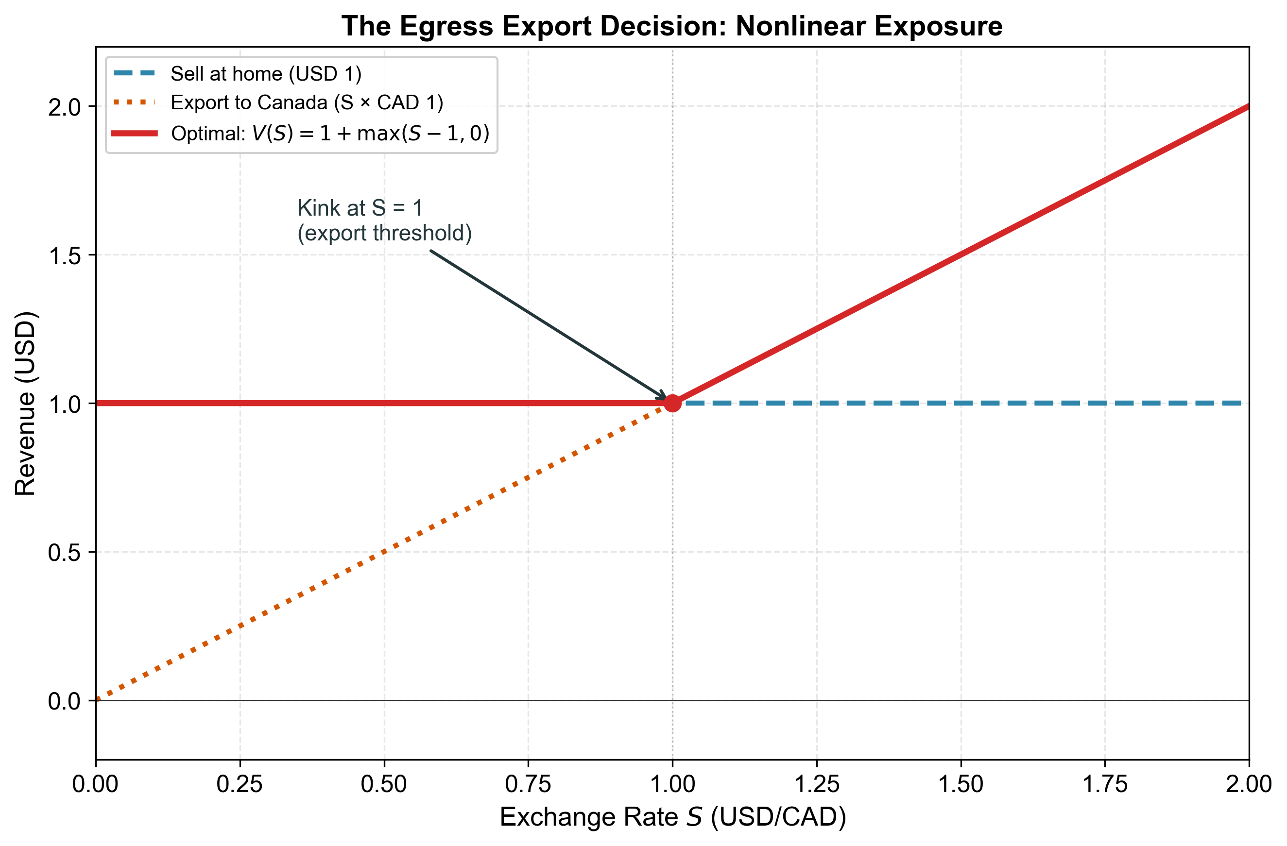
When exposure is kinked or nonlinear, identify the option-like component:
The kink in operating exposure corresponds to a real business decision (export or not, enter market or not, adjust prices or not)
The strike price of the embedded option is the threshold at which the decision changes
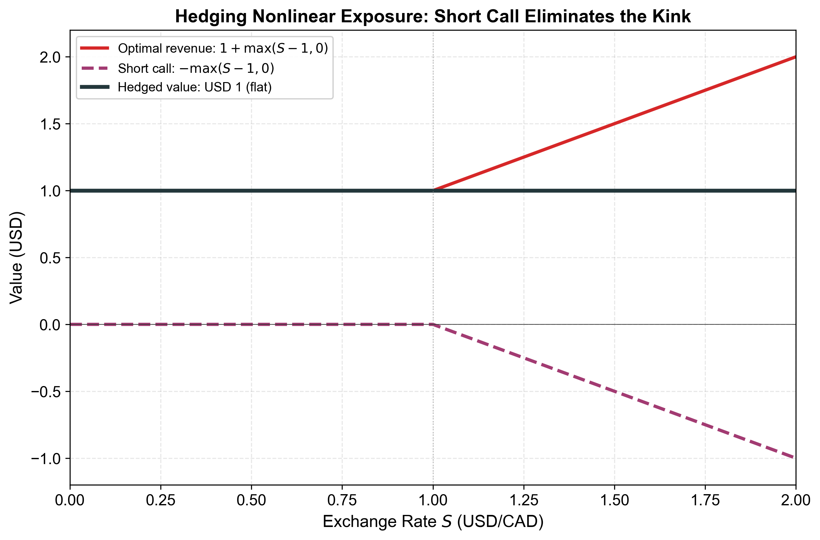
Hedge with the matching option (call or put, appropriate strike)
The operating flexibility of the firm IS an option — and option pricing theory tells us how to value and hedge it.
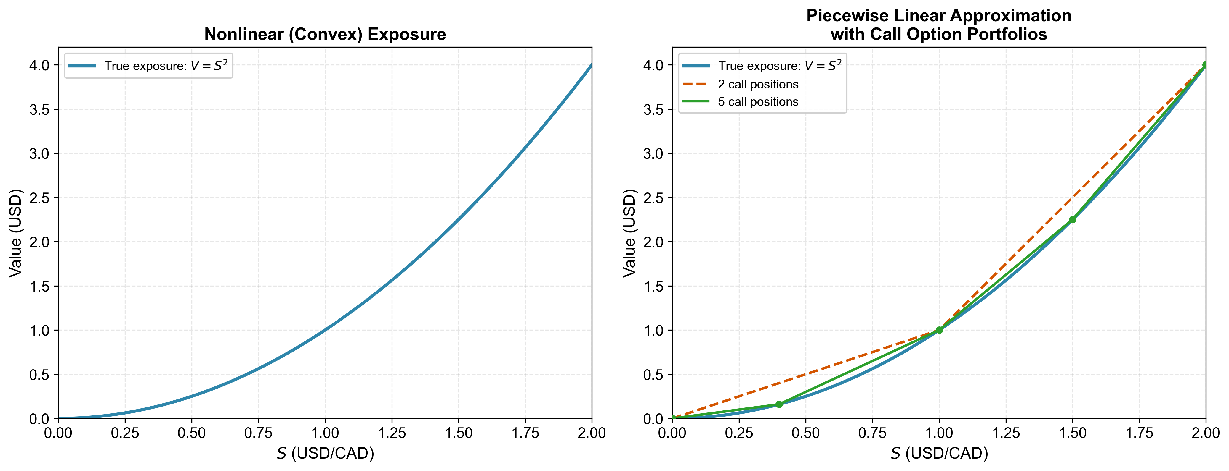
Approximating Smooth Nonlinear Exposure
Smooth nonlinearity
Not all exposures have a clean kink. Some are smoothly curved.
Example: Both export quantity AND price increase with \(S\):
\[V(S) = S \times S = S^2\]
This is convex exposure — the slope increases as \(S\) rises.
A single forward (linear) cannot capture the curvature.
Piecewise linear approximation
Practical implications
Any smooth curve can be approximated by a portfolio of calls at different strikes
Each call adds a kink, changing the slope — more calls means better fit
In practice:
Most firms don’t need perfect replication — 1-2 options can capture the main nonlinearity
Key question: where is the kink in your exposure? That determines the strike price.
If exposure is approximately linear over the relevant range \(\Rightarrow\) use a forward (simpler, cheaper)
If there’s a threshold, cliff, or significant curvature \(\Rightarrow\) use options
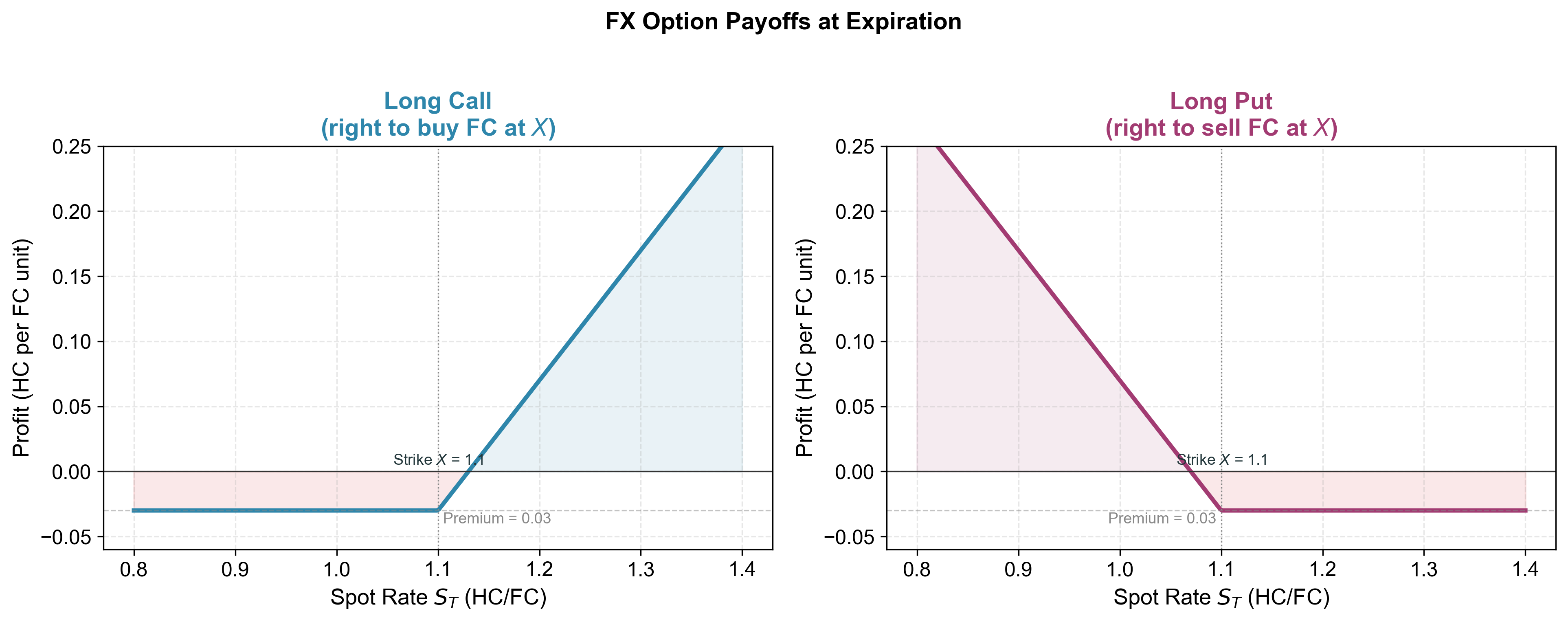
FX Option Strategies
Call and put payoffs
Call = right to buy FC at strike \(X\). Hedges FC outflows (caps the cost).
Put = right to sell FC at strike \(X\). Hedges FC inflows (sets a floor).
Cost: premium paid upfront (unlike forwards, which cost nothing to enter).
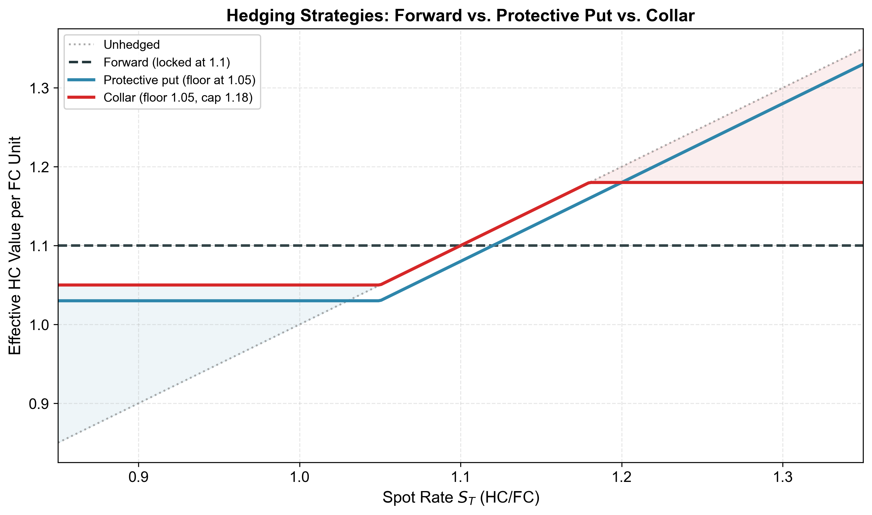
Strategy 1: Protective put (the floor)
Firm will receive FC\(\Rightarrow\) buys a put to set a floor on HC value.
If \(S_T < X\): exercise put, receive \(X\) per FC unit (protected)
If \(S_T > X\): let put expire, convert at market rate (upside preserved)
Outcome: downside protected, upside preserved.
Cost: option premium (paid upfront). This is the price of asymmetric protection.
The protective put is the simplest and most common option strategy for corporate hedging.
Strategy 2: Collar
Buy a put (floor) AND sell a call (cap) on the same FC amount.
The call premium received offsets (part of) the put premium paid
Zero-cost collar: choose strikes so premiums exactly offset
Outcome: bounded range — protected below the put strike, capped above the call strike. Trade-off: give up upside to reduce cost.
Strategy 3: Risk reversal
Buy OTM put (deep downside protection) + sell OTM call (give up far upside).
Near-zero premium: the call premium funds the put
Provides cheap tail protection against extreme adverse moves
Common in practice for event risk (elections, central bank decisions, geopolitical shocks)
Key insight: The risk reversal lets the firm insure against disaster scenarios while paying very little upfront — at the cost of giving up gains in the best-case scenarios.
When to use options vs. forwards
Use forwards when: exposure is certain (known amount, known date), FX view is neutral, cost minimization is the priority.
Use options when:
Exposure is uncertain or contingent (tenders, bids)
Exposure is nonlinear (thresholds, pricing power kinks)
Event risk is high (elections, regime changes)
Firm wants downside protection with upside participation
Layered hedging: forwards for near-term certain flows + options for tail risk or uncertain flows further out.
Tender hedging: the classic option application
Setup: Firm submits a bid in FC for a contract.
If it wins: FC inflow. If it loses: nothing.
Forward hedge is dangerous: if bid rejected, firm has a naked forward position (must deliver FC it doesn’t have).
Put option solves this:
If bid accepted \(\Rightarrow\) exercise put to lock in exchange rate
If bid rejected \(\Rightarrow\) let put expire (lose premium only)
This is why option markets exist for corporates — they hedge contingent exposures where the amount itself is uncertain.
FX Option Pricing
The Garman-Kohlhagen formula
The Black-Scholes model adapted for FX (Garman-Kohlhagen, 1983):
Uses the forward rate\(F\) as the underlying (accounts for interest rate differential via CIP)
Key input: volatility\(\sigma\) — the only unobservable
What drives option prices
Five inputs determine the option price (table holds the forward \(F\) fixed when varying \(r\)):
Input
Effect on call
Effect on put
Forward rate \(F\)\(\uparrow\)
\(\uparrow\)
\(\downarrow\)
Strike \(X\)\(\uparrow\)
\(\downarrow\)
\(\uparrow\)
Volatility \(\sigma\)\(\uparrow\)
\(\uparrow\)
\(\uparrow\)
Time to expiry \(T\)\(\uparrow\)
\(\uparrow\)
\(\uparrow\) (\(^*\))
HC interest rate \(r\)\(\uparrow\) (holding \(F\) fixed)
\(\downarrow\)
\(\downarrow\)
\(^*\) Generally true for plain European options; can be affected by rates/carry in edge cases.
Note on the rate row. If instead spot \(S_0\) and \(r^*\) are held fixed, a higher domestic rate \(r\)raises the forward\(F\), which tends to raise calls and lower puts. The table separates this forward effect from the pure-discounting effect.
Volatility is the critical input: higher vol \(\Rightarrow\) more expensive options. The forward rate (not spot) is the natural underlying — this connects back to CIP (Lecture 4).
Put-call parity in FX
A call and put with the same strike and expiry are linked by arbitrage:
\[c - p = \frac{F - X}{1 + r}\]
If you know the call price, you get the put price for free (and vice versa)
A forward is equivalent to: long call + short put at strike \(F\)
At-the-money forward (\(X = F\)): \(c = p\) (call and put have equal value)
Put-call parity is a no-arbitrage condition — it holds by the same logic as CIP.
Replication and delta
An option can be replicated by a dynamic portfolio of a forward + a bond
The hedge ratio (delta, \(\Delta\)) tells you how many forwards you need:
Call delta: between 0 and 1
Put delta: between \(-1\) and 0
Key difference from forwards:
A forward has constant delta = 1
An option has changing delta — it varies with \(S\)
This connects to the nonlinear exposure discussion: the changing delta of an option is what allows it to match nonlinear exposure that a constant-delta forward cannot.
The call’s exposure is \(\frac{1}{3}\) of a forward — it moves \(\frac{1}{3}\) as much as the spot rate.
Step 2 — Bond position: From the down-state equation: \[B = \frac{0 - \tfrac{1}{3}(950 - 1009.6)}{1.05} = \frac{19.87}{1.05} \approx 18.92\]
Step 3 — Call price: Cost of replicating portfolio (forward costs zero to enter):
\[c_0 = B \approx 18.92\]
Key insight: We priced the option without knowing the true probability of up/down. Only the no-arbitrage condition and the ability to replicate matter.
Risk Information in Option Prices
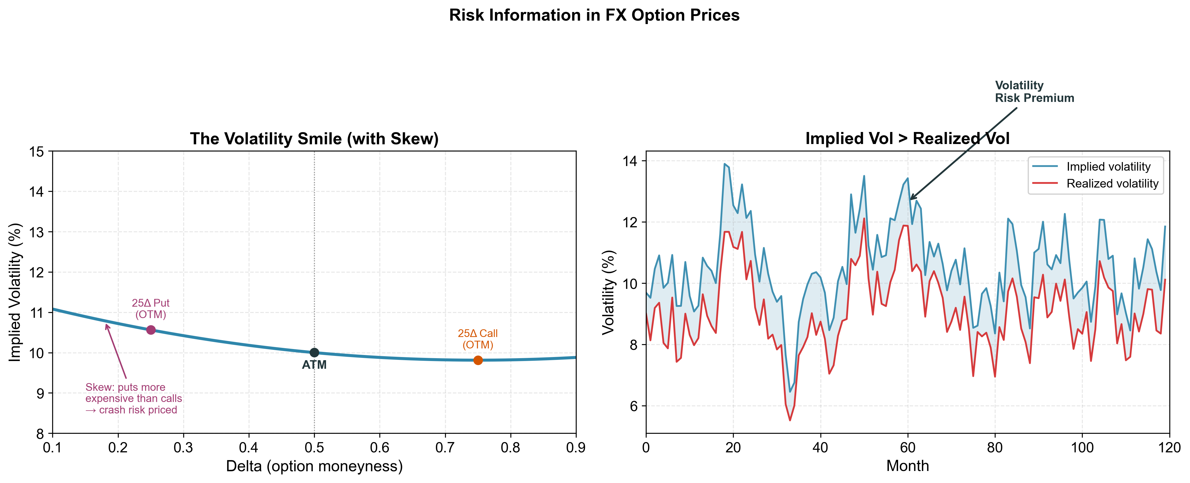
Implied volatility
Given an observed option price, invert the GK formula to extract the market’s expectation of future volatility.
This is implied volatility (\(\sigma_{\text{imp}}\)):
Option sellers earn a premium for bearing volatility risk
The wedge is the volatility risk premium (VRP)
VRP = compensation for the risk that volatility spikes unexpectedly
Why it matters: When a firm buys a put to hedge, it pays the VRP on top of “fair” value. Hedging with options is more expensive than a pure probability calculation would suggest — because the seller demands compensation for risk.
Risk reversals as sentiment indicators
Risk reversal = IV of 25\(\Delta\) call \(-\) IV of 25\(\Delta\) put
Positive RR: calls more expensive \(\Rightarrow\) market expects FC appreciation
Negative RR: puts more expensive \(\Rightarrow\) market expects FC depreciation
Corporate treasurers and traders use risk reversals as a real-time sentiment gauge:
A sharp move in the RR signals changing market expectations
Useful for timing hedge decisions (though not for speculation!)
Risk reversals are quoted directly in the interbank FX options market — they are one of the primary instruments traded.
Connection to course themes
The volatility risk premium is observable evidence that FX risk is priced.