Three types of exposure: transaction, translation, operating
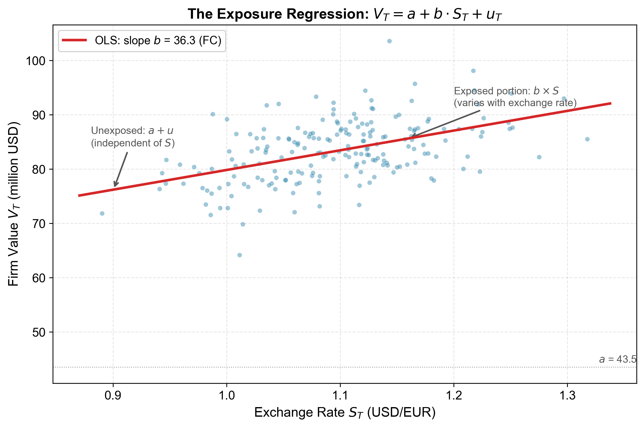
The exposure regression: \(V = a + bS + u\)
Operating exposure examples and measurement
Hedging with forwards: transaction and operating exposure
Multiple FC cash flows: aggregation and hedging
Overview of hedging instruments
From “Why Hedge” to “What to Hedge”
Recap and transition
Lecture 6 established:
Under M&M, hedging is irrelevant
In reality, hedging adds value through: distress costs, tax convexity, agency costs, information asymmetries
But to hedge, you first need to measure what you’re exposed to.
This lecture answers: What is exposure, how do we measure it, and how do we hedge it?
Risk vs. exposure
Exchange rate risk = uncertainty about the future spot rate.
Same for all firms. Determined by the market.
Exchange rate exposure = how much firm value changes per unit change in the exchange rate.
Firm-specific. Depends on the firm’s business, contracts, and competitive position.
Two firms in the same country, facing the same FX risk, can have very different exposures — one may benefit from a depreciation while the other is harmed by it.
Three Types of Exposure
Overview
Transaction exposure: known FC-denominated contractual cash flows
Exposed portion (\(b \times S_T\)): varies with the exchange rate. Can be hedged.
Unexposed portion (\(a + u_T\)): independent of the exchange rate. Cannot be hedged with FX instruments.
Units:
\(V_T\)
\(a\)
\(b\)
\(S_T\)
\(u_T\)
HC
HC
FC
HC/FC
HC
The exposure \(b\) is in foreign currency units — it is the FC amount you need to hedge.
Interpreting the exposure coefficient
\(b > 0\): firm benefits from FC appreciation (net exporter profile, long FC)
\(b < 0\): firm benefits from FC depreciation (net importer profile, short FC)
\(b = 0\): firm is not exposed to this exchange rate
Estimating \(b\) in practice:
Regression approach: regress stock returns on FX changes: \(r_{i,t} = \alpha + \beta \cdot \Delta s_t + \varepsilon_t\)
Scenario analysis: project cash flows under different FX assumptions
The regression approach captures all channels (transaction + translation + operating). But \(\beta\) may be noisy, time-varying, and affected by existing hedges.
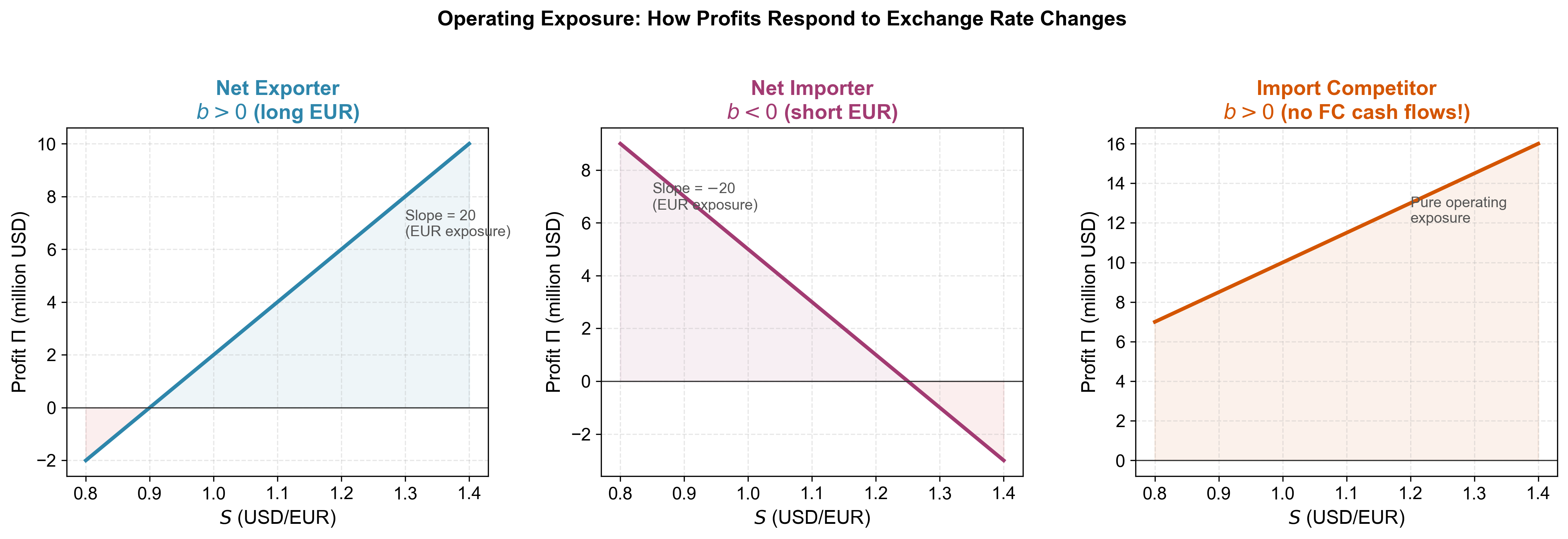
Operating Exposure Examples
Net exporter
Revenue in FC, costs in HC
HC depreciation (\(S \uparrow\)): FC revenues worth more in HC terms \(\Rightarrow\) profits rise
Exposure \(b > 0\) (long FC)
Profit function:
\[\Pi(S) = b \cdot S - C_{\text{HC}}\]
Example: European pharmaceutical company selling drugs in USD. EUR revenues are fixed costs; USD revenues increase in EUR terms when EUR depreciates.
Net importer
Revenue in HC, costs in FC
HC depreciation (\(S \uparrow\)): FC costs rise in HC terms \(\Rightarrow\) profits fall
Example: US retailer sourcing products from Asia. Revenues are in USD; costs increase in USD terms when USD depreciates against Asian currencies.
Import competitor: the subtle case
Both revenues AND costs in HC — no explicit FC cash flows
But: competes with foreign firms whose costs are in FC
HC appreciation (\(S \downarrow\)): foreign competitors become cheaper \(\Rightarrow\) domestic firm loses market share
Exposure \(b > 0\) even though the firm has zero transaction exposure.
Example: US steel producer competing with Korean imports. All costs and revenues in USD. But when USD appreciates, Korean steel becomes cheaper in USD, taking market share.
This is pure operating exposure — invisible if you only look at contracts.
Profit functions
What determines the magnitude of operating exposure?
Pricing power: Can the firm pass through FX changes to customers?
Market structure: How competitive is the industry? More competition \(\Rightarrow\) larger operating exposure.
Cost structure: Domestic vs. imported inputs
Strategic flexibility: Can the firm shift production, sourcing, or pricing?
Time horizon: Operating exposure generally grows with the horizon
Firms with high pricing power and flexible operations have lower operating exposure. Commodity-like industries with intense competition have higher operating exposure.
Hedging with Forwards
Hedging transaction exposure
Setup: You will receive FC \(X\) at time \(T\).
Exposure = \(X\) (in FC)
Hedge: sell FC \(X\) forward at rate \(F_{t,T}\)
Hedged value:
\[V_T^H = X \times F_{t,T}\]
This is known today — no FX risk remains.
This is the simplest case. The forward contract exactly offsets the exposure because both the amount and the timing are known.
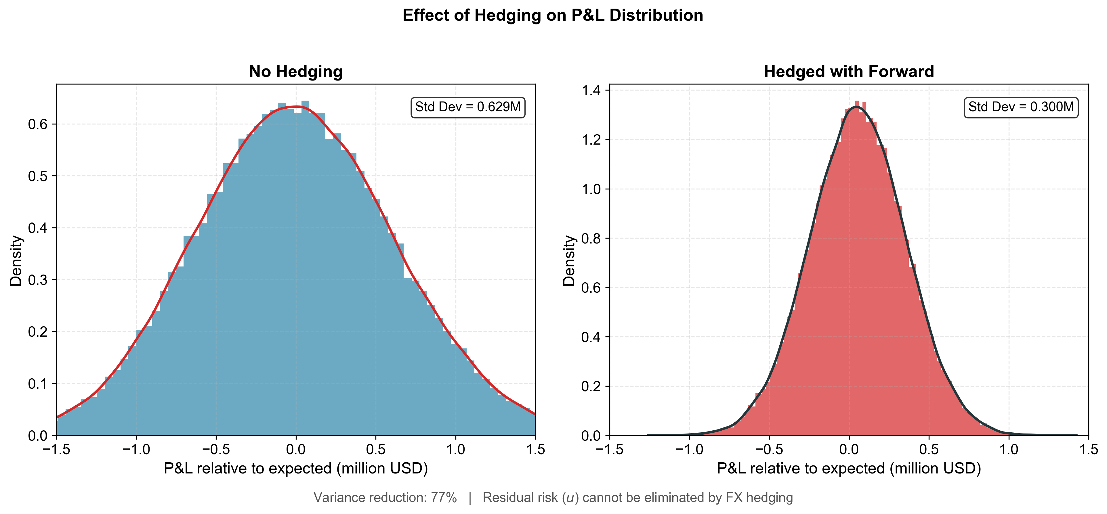
Hedging operating exposure
From the regression: exposure = \(b\) (in FC units).
Hedge: sell FC \(b\) forward at rate \(F_{t,T}\).
Hedged value:
\[V_T^H = a + b \times F_{t,T} + u_T\]
The FX risk (\(b \times S_T\)) is replaced by a known quantity (\(b \times F_{t,T}\))
Residual risk\(u_T\) remains — it cannot be hedged with FX instruments
Warnings about hedging operating exposure
Exposure \(b\) is estimated, not observed \(\Rightarrow\) hedge is approximate
Exposure changes over time\(\Rightarrow\) hedge needs updating (dynamic hedging)
Residual risk \(u_T\) can be substantial
Financial hedging alone may be insufficient for operating exposure
Operational hedges may be needed:
Diversify production locations (match FC costs with FC revenues)
Diversify sourcing across currencies
Build flexibility into pricing and contracts
Best practice: Use financial hedges for near-term known flows (transaction exposure) and operational hedges for longer-term competitive effects (operating exposure).
Multiple FC Cash Flows
Aggregating exposure across maturities
A firm may have FC cash flows at different dates:
\[X_1 \text{ at } T_1, \quad X_2 \text{ at } T_2, \quad \ldots, \quad X_n \text{ at } T_n\]
Cannot simply add them — different maturities have different present values.
Aggregate exposure = present value of all FC cash flows:
The duration-matched hedge is an : it matches the PV sensitivity of the cash-flow stream to FX moves, but it is not identical to hedging each dated cash flow separately. The forward notional is the future value of the GBP PV at the hedge date, not the PV itself — the two coincide only when \(r_{\text{GBP}} = 0\).