International Finance

Purchasing Power Parity and Real Exchange Rates

Main issues

• Does exchange rate risk exist?

• Purchasing power parity: absolute and relative

• Empirical evidence across horizons

• The real exchange rate and why PPP failure matters for firms

Does Exchange Rate Risk Exist?

The question

Is there exchange rate risk?

Most likely — but not necessarily.

If all prices adjust immediately and fully to exchange rate changes, then nominal FX movements have no real effect.

This is what Purchasing Power Parity claims.

The thought experiment

• USD/CAD = 1.00. An iPhone costs 650 USD in the US and 650 CAD in Canada.

• Exchange rate moves to 1.10 (CAD depreciates by 10%)

• If the CAD price drops to \(650/1.10 = 590.91\), buying in either country still costs 650 USD

• This is PPP in action — prices adjust to offset the exchange rate move

Does this actually happen?

Apple and Brexit: a natural experiment

June 2016: GBP depreciates $$15% after Brexit referendum.

Apple raises UK prices weeks later:

	GBP Price	USD/GBP	Implied USD Price
May 2016 (pre-Brexit)	£499	1.45	$724
Sep 2016 (post-Brexit)	£549	1.33	$730

Some pass-through happened — but it took weeks, was incomplete, and was a discrete jump.

Not the smooth continuous adjustment PPP assumes.

The real exchange rate

Define the real exchange rate:

\[e_t = S_t \cdot \frac{P^*_t}{P_t}\]

where \(S_t\) is the nominal rate (HC/FC), \(P_t\) is the HC price level, \(P^*_t\) is the FC price level.

• If PPP holds: \(e_t = 1\) (or constant)

• If \(e_t\) moves: there is real exchange rate risk

Preview: \(e_t\) is not constant. Not even close.

USD/GBP nominal exchange rate

Absolute PPP

Absolute PPP: definition

The exchange rate equals the ratio of price levels:

\[S_t = \frac{P_t}{P^*_t}\]

Rationale: If the equality does not hold, one could exploit “real” arbitrage on physical goods. Prices should be the same once converted to a common currency.

Example: If a good costs $0.50 in the US and NOK 1.50 in Norway:

\[\text{USD/NOK} = \frac{0.50}{1.50} = \frac{1}{3}\]

The Big Mac Index

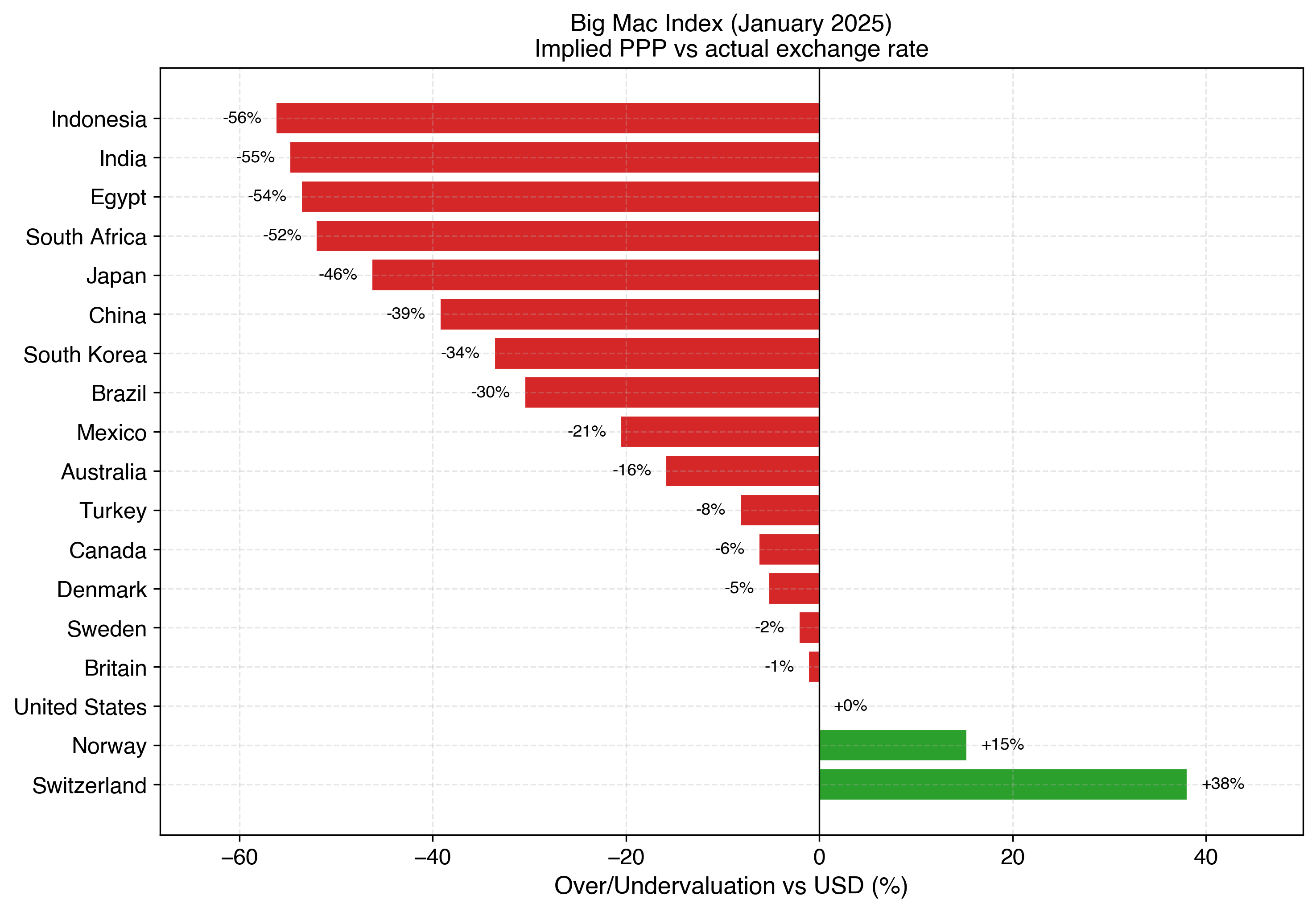
Source: The Economist, Big Mac Index (January 2025)

Classic test of absolute PPP for a single standardized good. Persistent deviations: Big Macs are “cheap” in emerging markets, “expensive” in Scandinavia/Switzerland. Partly Balassa-Samuelson.

Why absolute PPP fails

• Many goods are non-traded: high transport costs (cement, bricks), services (haircuts, healthcare)

• Even for traded goods: transport costs, tariffs, trade barriers create bands around PPP

• Only considers goods and services, not capital flows

• Balassa-Samuelson effect creates systematic deviations (next slide)

Conclusion: Absolute PPP — \(e_t = 1\) always — is too strong. We need to relax it.

Balassa-Samuelson effect (1964)

1. Productivity in traded goods is higher in developed countries than emerging economies

2. Productivity in non-traded services is similar everywhere (haircuts, taxis)

3. But wages equalize within a country across sectors — so non-traded goods are expensive in rich countries

Example: A haircut costs $40 in Oslo and $15 in São Paulo — but the barbers are equally skilled.

Implication: Price levels are systematically higher in richer countries. Absolute PPP is biased.

This is exactly what the Big Mac Index shows.

Relative PPP

Relative PPP: definition

Exchange rate changes should be proportional to relative inflation:

\[S_1 = \frac{P_1/P_0}{P^*_1/P^*_0} \cdot S_0\]

Log-differenced version:

\[\Delta s_t \approx \pi_t - \pi^*_t\]

This relaxes the level condition — only requires changes to offset.

Relative PPP: rationale and prediction

Rationale:

• Higher inflation at home \(\rightarrow\) home currency depreciates

• Depreciation compensates foreign buyers for higher domestic prices

Prediction:

• If domestic prices rise 50% and foreign prices are flat, the domestic currency should depreciate 50%

What it does NOT require: That price levels are equalized across countries (unlike absolute PPP)

Why relative PPP also fails

• Does not account for structural changes (wars, regime shifts, financial crises)

• Balassa-Samuelson applies here too: if one country is growing faster, its non-traded prices rise faster, creating a secular trend

• Works better at very long horizons (decades) but poorly at business-cycle frequencies

How badly does it fail? Let’s look at the data.

Empirical Evidence

Actual vs. PPP-implied exchange rate

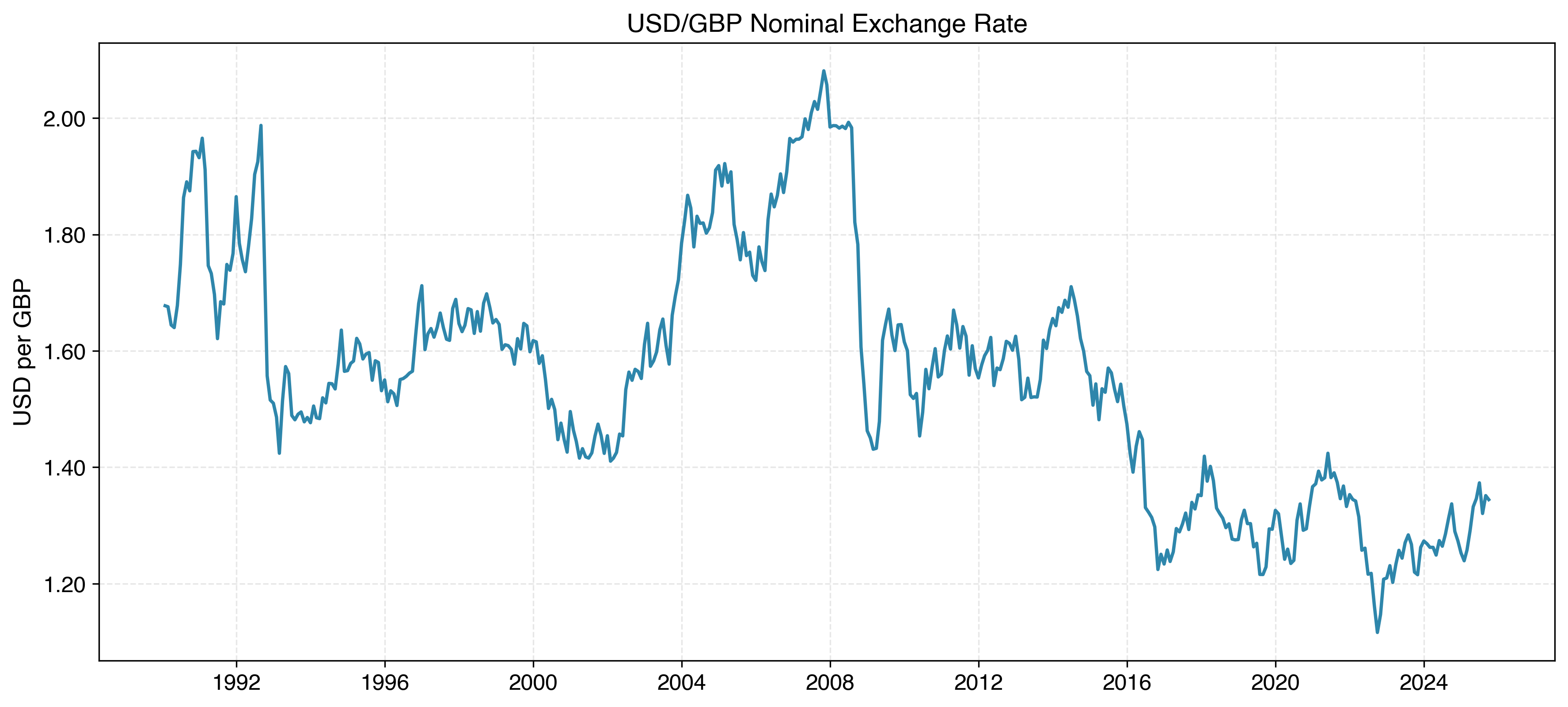
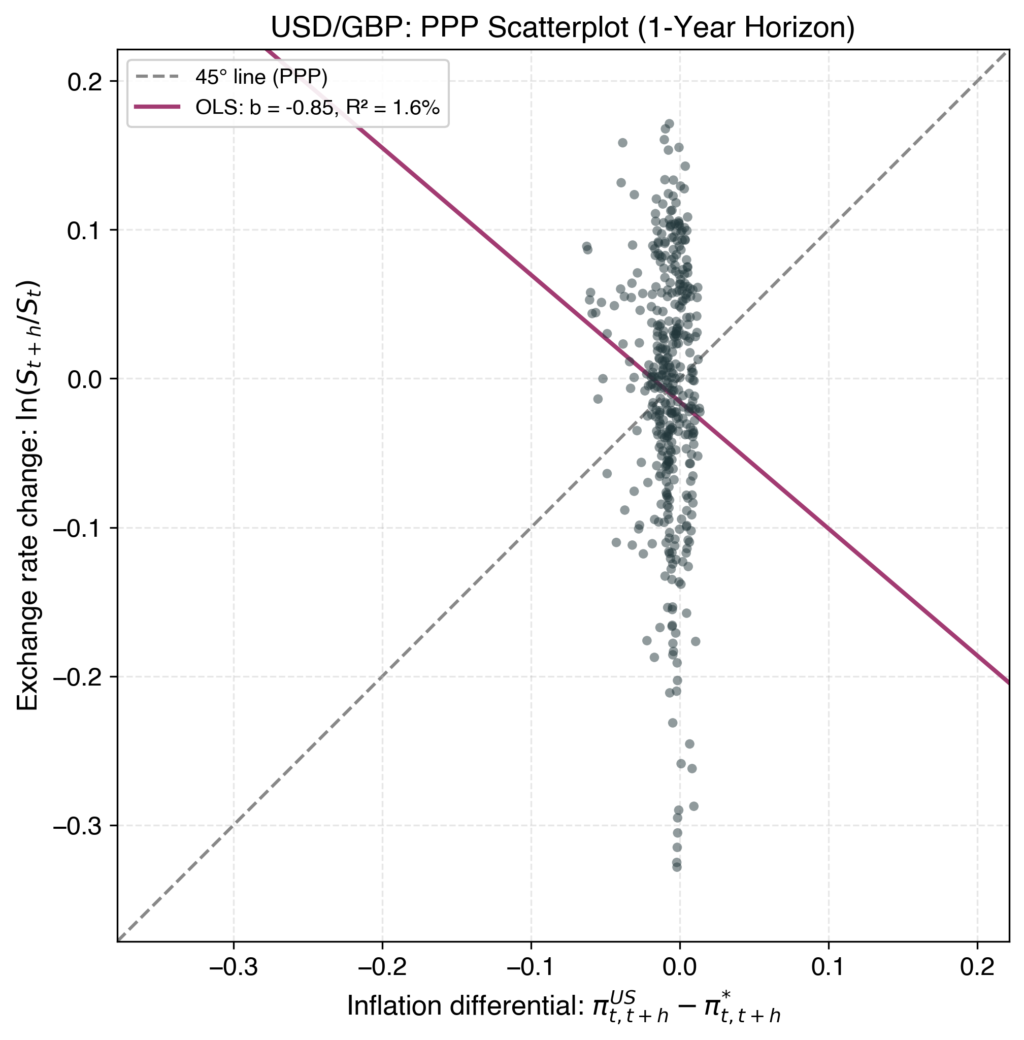
Data: 1990–2025. PPP-implied rate uses cumulative US vs UK inflation from base period.

Massive, persistent deviations lasting years. The PPP-implied rate drifts slowly; the actual rate swings widely around it. GBP was overvalued vs PPP for most of 2003-2008 (pre-crisis), then sharply undervalued.

PPP regression test: setup

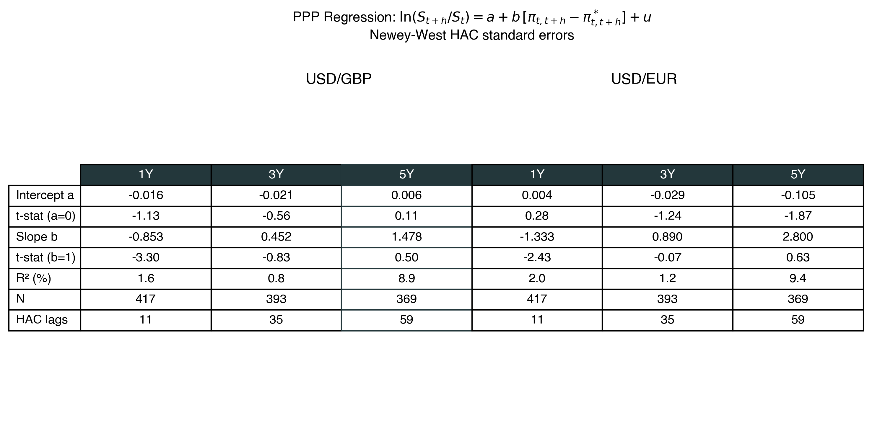
Regression:

\[\ln\frac{S_{t+h}}{S_t} = a + b\left[\pi^{US}_{t,t+h} - \pi^{UK}_{t,t+h}\right] + u_{t+h}\]

PPP null hypothesis: \(a = 0\) and \(b = 1\)

• Test at multiple horizons: \(h \in \{1, 3, 5\}\) years

• Forward-looking inflation: \(\pi_{t,t+h} = \ln(P_{t+h}/P_t)\)

• Newey-West HAC standard errors (overlapping observations)

PPP regression results

Interpreting the results

• Short horizon (1Y): \(R^2 \approx 0\), slope far from 1 \(\rightarrow\) PPP has no predictive power

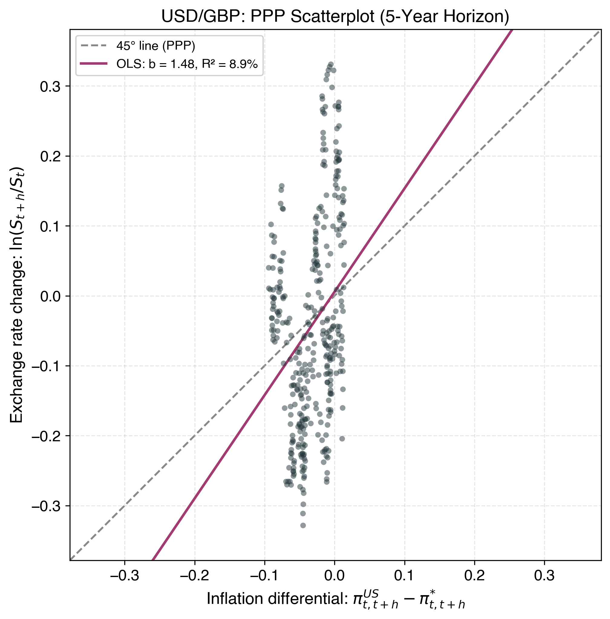
• Medium horizon (3Y): \(R^2\) improves, slope moves toward 1 \(\rightarrow\) slow convergence

• Long horizon (5Y): \(R^2\) rises further \(\rightarrow\) PPP gains explanatory power but remains noisy

Same pattern for USD/EUR — this is not a GBP-specific result.

The PPP puzzle (Rogoff 1996): Deviations have half-life of 3–5 years. Too slow for nominal rigidities alone. Too fast for purely real shocks.

PPP scatterplot: 1-year horizon

At the 1-year horizon the scatter is essentially a cloud — inflation differentials explain almost nothing about exchange rate movements. This is the PPP puzzle in action.

PPP scatterplot: 5-year horizon

At 5 years the relationship begins to emerge but remains noisy. The slope moves toward 1 and R² increases, consistent with slow mean reversion. PPP has more explanatory power at longer horizons, but deviations remain large.

The Real Exchange Rate

Real exchange rate over time

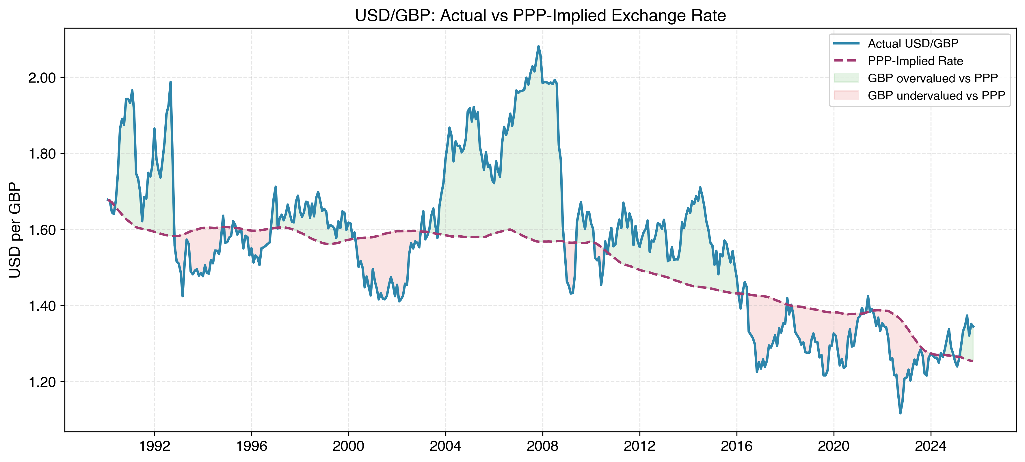
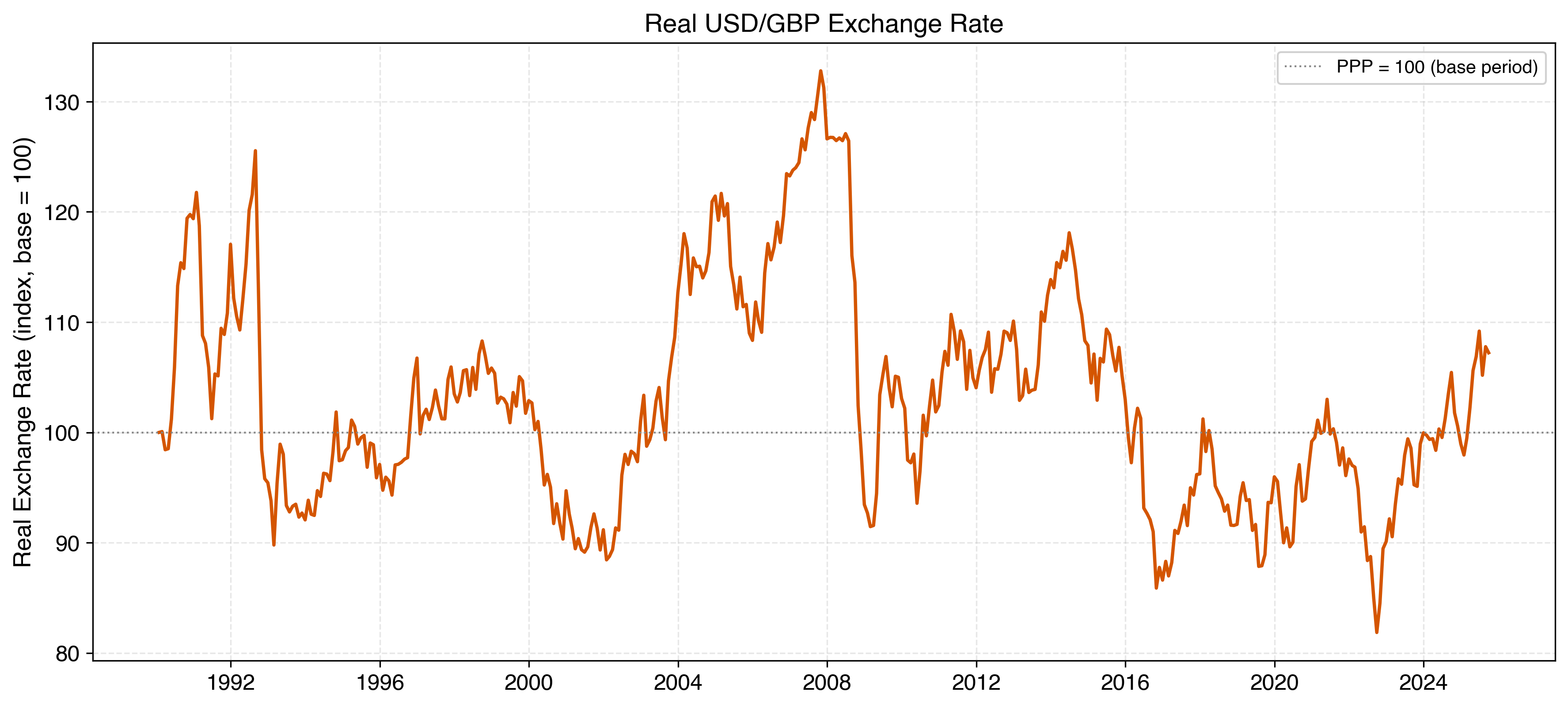
Real USD/GBP = \(S_t \cdot P^{UK}_t / P^{US}_t\), indexed to 100 at start of sample.

What the real exchange rate tells us

• Swings of \(\pm 30\%\) lasting years — not noise

• Mean-reverting over decades but not at business-cycle frequencies

• Each swing represents a period where goods are genuinely cheaper or more expensive across countries

When the real rate rises: Foreign goods become expensive relative to domestic. Domestic exporters gain competitiveness.

When the real rate falls: The reverse. Domestic firms face margin compression from foreign competition.

Why this matters for the firm

PPP failure means nominal FX changes have real effects:

• Revenue in FC may not be offset by cost changes

• Competitive position shifts with the real exchange rate

  • A German automaker vs. a Japanese rival: EUR/JPY matters in real terms

• Margin compression, volume changes, supply chain costs

This is the bridge from Layer 1 to Layer 3:

• Real FX risk \(\rightarrow\) operating exposure (Lecture 4)
• Real FX risk \(\rightarrow\) affects expected CFs in cross-border valuation (Lectures 7–8)

Key takeaways

• Absolute PPP fails: non-traded goods, transport costs, Balassa-Samuelson

• Relative PPP works only at very long horizons (decades, not years)

• Real exchange rate risk is persistent and economically large (\(\pm 30\%\))

• For the firm: FX exposure is real, not just nominal — this is why hedging, financing, and investment decisions are hard

CF vs. DR: PPP failure is primarily a cash flow effect — it changes real revenues, margins, and competitive position.

Where this fits in the course

• PPP failure motivates the entire corporate block:

  • If PPP held, why hedge? \(\rightarrow\) Risk management (Lectures 4–5)
  • If PPP held, does borrowing currency matter? \(\rightarrow\) Financing (Lecture 6)
  • If PPP held, are foreign CFs risky? \(\rightarrow\) Investment (Lectures 7–9)

• Next lecture: CIP, UIP, and the forward rate — from goods-market parity to financial-market parity

Other exchange rate models exist (monetary approach, Dornbusch overshooting, portfolio balance) — they all perform poorly at short horizons. We focus on what matters for the firm.