International Finance

Country Risk: Measurement, Valuation, and Modern Challenges

Main Issues

• What is country risk and why does it matter for cross-border valuation?
• How to measure country risk: spreads, ratings, insurance

• The 500bp fallacy: why adjusting the discount rate is wrong
• Three methods for adjusting cash flows

• Modern country risk: sanctions, ESG/climate, BEPS Pillar Two
• Connection: completes the APV framework from Lectures 10–11

This lecture completes the cross-border valuation toolkit. Lecture 10 gave us the APV structure, Lecture 11 gave us the discount rate via ICAPM. This lecture addresses the remaining piece: how to handle country risk. The key message is that country risk should be reflected in cash flows, not the discount rate.

Part 1: What Is Country Risk?

We start with definitions and taxonomy, then move to measurement, the critical 500bp fallacy, and practical methods for incorporating country risk into valuation.

Where We Left Off

• Lecture 10: APV framework for cross-border valuation

  • Step 1: Base-case NPV (all-equity, no country risk)
  • Step 2: + Tax shields
  • Step 3: + Financing side effects
  • Step 4: – Country risk adjustment \(\leftarrow\) this lecture

• Lecture 11: ICAPM gave us the discount rate for Step 1

• Missing piece: How do we quantify and adjust for country risk?

Lecture 10 explicitly left Step 4 as a placeholder. Lecture 11 solved the discount rate question using the ICAPM and factor models. Now we need to handle the country-specific risks that can destroy cash flows.

Definition: Country Risk

Country risk is the risk that country-specific events destroy value of a cross-border investment

• Not a single risk — it’s an umbrella term for multiple, correlated risks
• Can affect cash flows, asset values, or the ability to repatriate profits
• Range from gradual regulatory changes to sudden expropriation

Key distinction: some country risks are systematic (priced by the market), others are idiosyncratic (diversifiable but can still destroy a project)

The definition is deliberately broad. Country risk encompasses everything from a minor tax change to a full-blown expropriation. The key analytical challenge is deciding which risks affect the discount rate (systematic) and which should be reflected in expected cash flows (idiosyncratic or partly diversifiable).

Three Levels of Country Risk

It helps to distinguish three layers:

1. Sovereign default risk: the probability that the government fails to pay its debts
   • Measured by sovereign bond spreads and credit ratings

2. Broader country risk: the full range of political, regulatory, and macro events that can destroy value
   • Sovereign default is one component, but far from the only one

3. Project-specific exposure: how much a particular investment is affected
   • An export-oriented mine and a domestic retailer face very different country risk in the same country

Sovereign spreads are informative but not a sufficient statistic for country risk

This distinction matters throughout the lecture. Sovereign spreads are the most commonly cited measure, but they only capture one dimension — sovereign creditworthiness. A country can have low sovereign default risk but high expropriation risk (e.g., resource nationalism in a fiscally strong country). And even within a country, different projects have very different exposures. Keep these three layers in mind as we discuss measurement and valuation methods.

Taxonomy of Country Risk

Five types of country risk: Transfer risk (capital controls, blocked repatriation), sovereign/expropriation risk (asset seizure, rule changes), political risk (regime change, conflict), currency/macro risk (inflation, currency collapse), and sanctions risk (a modern addition). The key insight at the bottom is crucial: these risks are correlated. A political crisis often triggers a currency collapse, which leads to capital controls. Russia 2022 is the perfect illustration of all five hitting simultaneously.

Country Risk Is Correlated

A single event can trigger cascading risks:

1. Political crisis (regime change, invasion, revolution)
2. \(\rightarrow\) Currency collapse (capital flight, loss of confidence)
3. \(\rightarrow\) Capital controls (government blocks outflows)
4. \(\rightarrow\) Regulatory changes (new taxes, local ownership rules)
5. \(\rightarrow\) Expropriation (nationalization of assets)

• Russia 2022: all five stages occurred within months
• This correlation means diversification across risk types doesn’t help — you need country diversification

This is why country risk is so dangerous. You can’t just insure against expropriation and feel safe, because the political crisis that leads to expropriation also brings currency collapse, capital controls, and regulatory changes. The only real hedge is geographic diversification of your project portfolio.

Part 2: Measuring Country Risk

Four main approaches to measuring country risk: sovereign bond spreads, credit ratings, political risk indices, and insurance premiums. Each has strengths and weaknesses.

Sovereign Bond Spreads

The most commonly used market-based measure:

• Compare yield on sovereign bond to US Treasury of same maturity
• Spread = sovereign yield \(-\) Treasury yield
• Reflects market’s assessment of default probability

Example

	Yield
One-year sovereign bond	13%
One-year US Treasury	6%
Spread	7%

• Higher spread \(\rightarrow\) higher perceived default risk
• Spreads move in real time as conditions change

Sovereign bond spreads are the workhorse measure. They’re market-based, forward-looking, and available in real time. The example uses the same numbers from the old slides: 13% sovereign yield minus 6% Treasury yield equals a 7% spread.

Emerging Market Credit Spreads Over Time

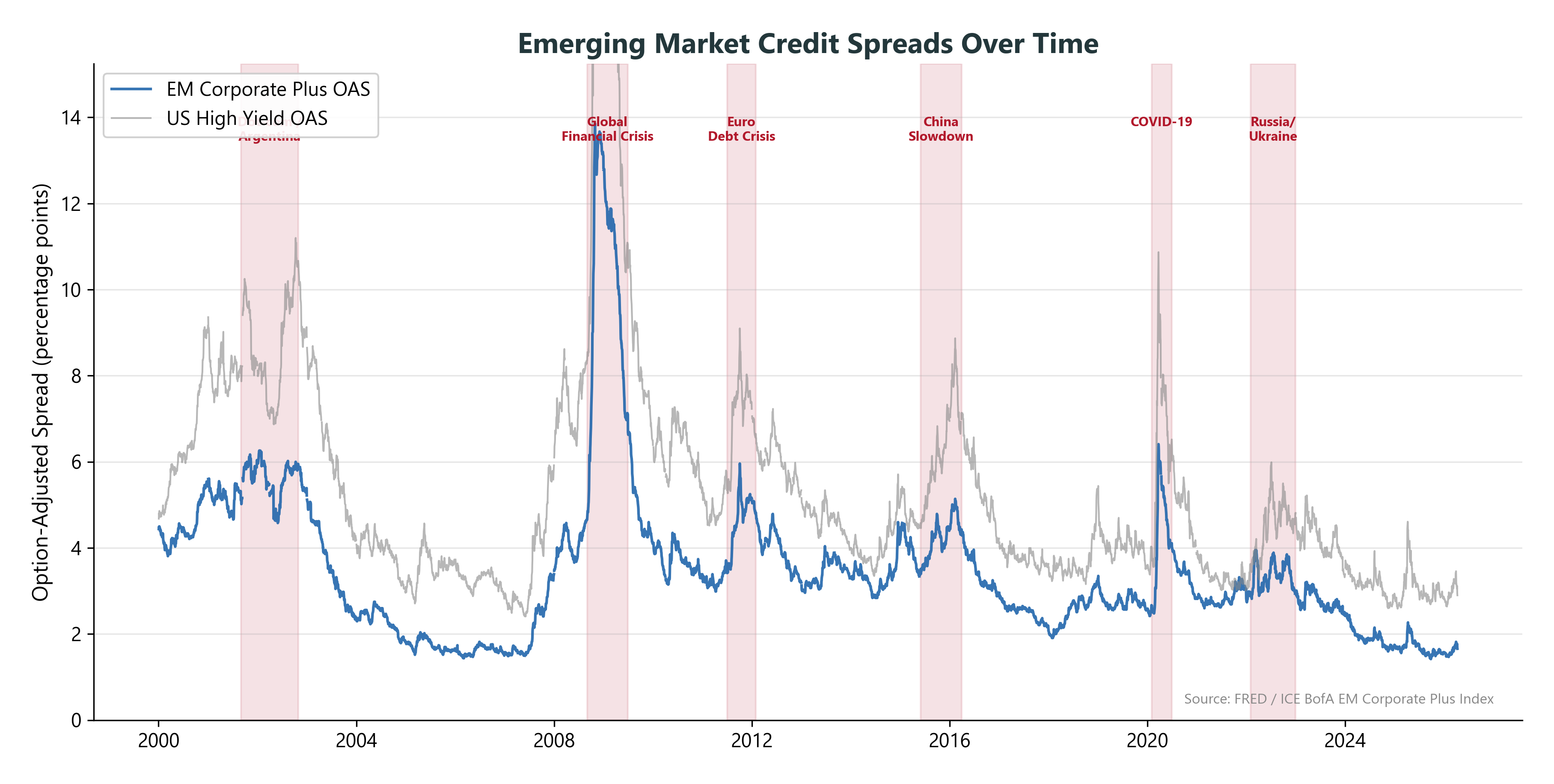
This shows emerging market corporate credit spreads (option-adjusted spread on the ICE BofA EM Corporate Plus Index) from FRED. These are corporate spreads, not sovereign spreads, but they track the same underlying country risk dynamics and spike during the same crises. Notice the 2001 Argentine default and dot-com bust, the massive GFC spike in 2008-09, the Euro debt crisis, the China slowdown scare in 2015-16, COVID-19, and the Russia/Ukraine shock. Key observation: spreads can go from 3% to 10%+ in a matter of weeks. This means country risk is time-varying, not a fixed constant you plug into your WACC.

From Spreads to Default Probability

The spread implies a market-priced default probability:

• Sovereign bond promises \(\$113\) (at 13% yield)
• Market values it at \(\$106\) (= \(\$100 \times 1.06\), the Treasury return)
• If default means total loss (recovery = 0):

\[(\$0 \times p) + (\$113 \times [1-p]) = \$106\]

\[p = 1 - \frac{106}{113} = 6.19\%\]

• With 5% recovery rate: \(p = \frac{113 - 106}{113 - 5.65} = 6.52\%\)
• This default probability is the key input for CF adjustment methods

This is the bond-implied default probability calculation from the old slides. Promised cash flow is 113, expected cash flow is 106. If default means total loss, the probability of default is 1 minus 106/113, which equals 6.19%. In practice, recovery rates are rarely zero, so the actual default probability is slightly higher. We’ll use this number later when we adjust cash flows.

Other Measurement Approaches

Credit ratings (Moody’s, S&P, Fitch)

• Stable but lag market events (often downgrade after crisis)
• Useful for regulatory thresholds (investment mandates)

Political risk indices (ICRG, World Bank Governance)

• Forward-looking, granular (governance, corruption, rule of law)
• Subjective, updated infrequently

Insurance premiums (MIGA, Lloyd’s, export credit agencies)

• Most market-based and deal-specific measure
• Covers book value, not market value; sudden events covered best

Ratings are useful but slow. They often downgrade after the crisis has already happened, making them less useful for forward-looking valuation. Political risk indices like ICRG provide granular scores on things like government stability, corruption, and rule of law, but they’re subjective. Insurance premiums are probably the most useful because they’re market-priced and deal-specific, but they have important limitations: they cover book value, not market value, and they don’t cover gradual deterioration of the business environment.

Summary: Measurement Tools

Tool	Pros	Cons
Sovereign spreads	Market-based, real-time	Volatile, credit + liquidity mixed
Credit ratings	Standardized, stable	Lag events, coarse
Political risk indices	Granular, forward-looking	Subjective, infrequent
Insurance premiums	Deal-specific, market-priced	Book value, limited coverage

• In practice, use multiple measures together
• No single measure captures all dimensions of country risk

The takeaway is that no single measure is sufficient. Sovereign spreads are the most widely used but mix credit risk with liquidity premiums. Ratings are standardized but slow. Insurance premiums are the most practical for deal-level analysis. A good analyst combines all of these.

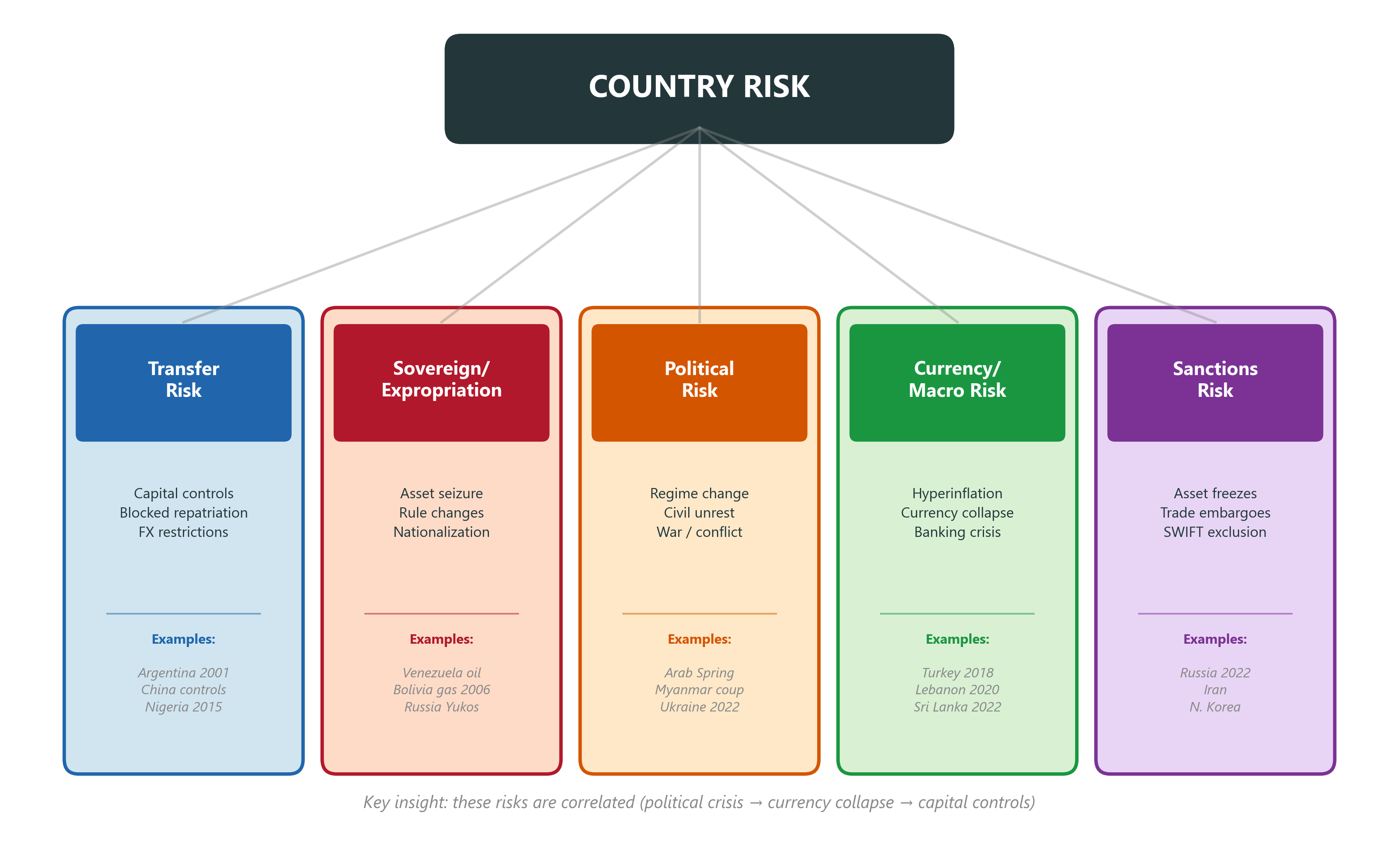
Part 3: The 500bp Fallacy

This is the most important conceptual section of the lecture. The common practice of adding a country risk premium to the discount rate is fundamentally flawed, and understanding why is critical for correct cross-border valuation.

Common Practice: Adjust the Discount Rate

Many practitioners simply add the sovereign spread to WACC:

• US project WACC: 10%
• Brazil sovereign spread: 5%
• Brazil project WACC: 10% + 5% = 15%

This is called the “500 basis point” approach

This is wrong. It’s convenient, widespread, and fundamentally flawed.

This is incredibly common in practice. Consulting firms, investment banks, and corporate finance teams routinely do this. It feels intuitive: riskier country, higher discount rate. But as we’ll see, it has at least five serious problems.

Why It’s Wrong: Problem 1 — Double-Counting

The sovereign spread is already reflected in local interest rates

• If you use the local risk-free rate to build your WACC, the spread is already there
• Adding it again means you’re counting country risk twice
• If you use the US risk-free rate + ICAPM (Lecture 11), you already have the systematic component

The ICAPM discount rate from Lecture 11 already prices whatever systematic component of country risk exists

This is the most basic problem. If your WACC calculation starts with the local risk-free rate (which already includes the sovereign spread), adding the spread again is pure double-counting. And if you’re using the US risk-free rate plus the ICAPM (as Lecture 11 recommends), then the systematic component of country risk is already captured by your world market beta and currency betas.

Why It’s Wrong: Problem 2 — Not All Projects Are Equal

Adding a uniform spread assumes all projects in a country face the same risk

But consider two projects in the same country:

Project	Country Risk Exposure
Export-oriented gold mine	Low: revenues in USD, global buyers
Domestic retail chain	High: local revenues, local regulation

• Same country spread, but very different country risk exposure
• The DR approach treats them identically — that’s wrong

An export-oriented mine earns revenues in hard currency from global buyers. Even if the country has a political crisis, the mine’s cash flows may be largely unaffected because the product is sold internationally. A domestic retail chain, on the other hand, is completely exposed to local economic conditions, currency controls, and consumer spending. Adding the same country risk premium to both projects makes no sense.

Why It’s Wrong: Problem 3 — Systematic vs Idiosyncratic

An important component of country risk is country-specific (diversifiable)

• Finance theory: only systematic risk deserves a risk premium in the discount rate
• Many country-specific events (a single sovereign default, a localized political crisis) are largely diversifiable for a global investor
• The ICAPM from Lecture 11 already captures whatever systematic component exists

However: market measures like spreads also embed global risk appetite, dollar liquidity conditions, and contagion effects — so observed spreads are not purely idiosyncratic

Implication: country risk should primarily affect expected cash flows, not the discount rate — but recognize that not all of it is purely diversifiable

This is the finance theory argument, but stated more carefully. The CAPM and ICAPM tell us that only systematic risk belongs in the discount rate. An important part of country risk is country-specific and diversifiable. But sovereign spreads are not pure measures of idiosyncratic risk — they move with global risk appetite (the VIX, dollar strength, Fed policy), meaning they embed a systematic component. The ICAPM betas from Lecture 11 already capture this systematic component. The remaining country-specific risk belongs in expected cash flows. The practical recommendation is the same — adjust cash flows, not the discount rate — but the reasoning is more nuanced than “country risk is purely idiosyncratic.”

Why It’s Wrong: Problem 4 — Ignores Deal Structure

Deal structuring can reduce country risk substantially:

• Political risk insurance (MIGA, Lloyd’s)
• Joint ventures with local government or international partners
• International arbitration clauses (ICSID)
• Revenue in hard currency, debt in local currency
• Key technology kept offshore (“Coca-Cola recipe”)

Adding a flat spread ignores all of these protections

This is a practical point. Companies don’t just passively accept country risk. They structure deals to minimize it. Joint ventures with local governments make expropriation less likely. International arbitration clauses provide legal protection. Revenue in hard currency reduces transfer risk. A flat spread on the discount rate ignores all of these deal-specific protections, treating a well-structured deal the same as an unprotected one.

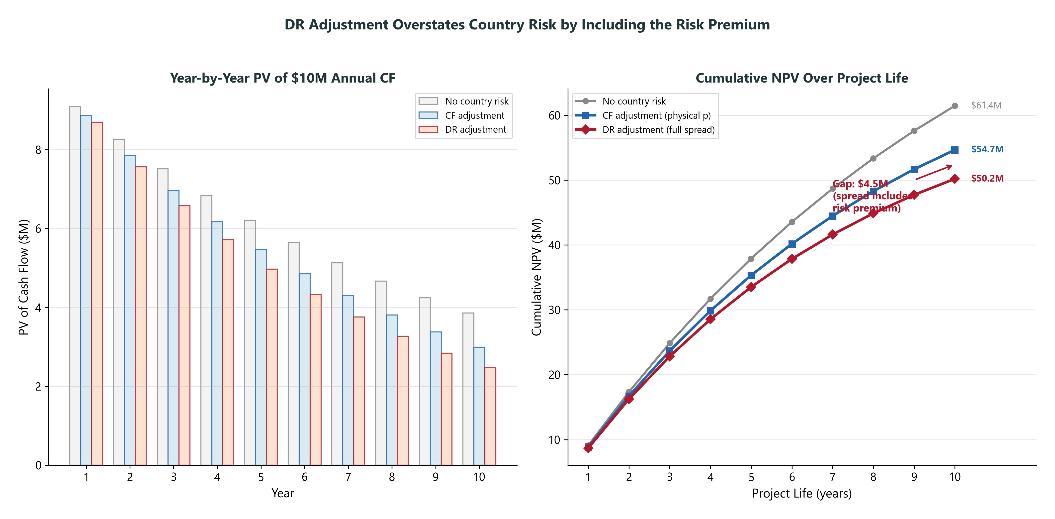
Why It’s Wrong: Problem 5 — Overstates Risk for Long-Lived Projects

Adding the full sovereign spread to the discount rate overstates country risk because the spread includes a risk premium above the actual expected loss

This figure compares the DR method (adding the full 5% spread to the discount rate) with the CF method (using a 2.5% physical default probability). Why 2.5%? Because the spread observed in bond markets is a risk-neutral measure that includes both expected loss AND a premium for bearing default risk. The physical (real-world) default probability — what you need for adjusting expected cash flows — is typically much lower than the risk-neutral probability implied by the spread. With consistent assumptions (same risk-neutral probability), the two methods would give identical results. The gap in the figure reflects the risk premium component of the spread, which the DR method incorrectly treats as expected loss. This bias grows with project life, penalizing infrastructure and mining investments.

The Right Approach

Separate the discount rate from country risk:

1. Discount rate: Use ICAPM from Lecture 11
   • Captures systematic risk only
   • World market beta, currency factor betas
   • No country risk premium added

2. Expected cash flows: Adjust for country risk
   • Scenario-weighted expected values
   • Reflects probability and severity of country-specific events
   • Deal-specific (accounts for insurance, JVs, etc.)

“Discount rate for systematic risk, cash flows for country risk”

This is the key takeaway. The discount rate handles systematic risk via the ICAPM. Country risk is handled by adjusting expected cash flows. This approach is theoretically correct (only systematic risk in the discount rate), practically flexible (accounts for deal structure), and doesn’t create the compounding bias against long-lived projects.

Part 4: Cash Flow Adjustment Methods

Three methods for incorporating country risk into cash flows: bond-implied default probability, scenario analysis, and APV with political risk insurance. Each has its place depending on the situation.

Method 1: Bond-Implied Default Probability

Use sovereign spreads to compute annual default probability, then “haircut” cash flows:

Step 1: Extract default probability from spread

• Spread = 4%, recovery rate = 5%
• \(p = \frac{\text{spread}}{1 - \text{recovery}} = \frac{0.04}{0.95} \approx 4.2\%\) per year

Step 2: Adjust each year’s cash flow

\[\text{Adjusted CF}_t = \text{Base CF}_t \times (1-p)^t\]

Step 3: Discount at ICAPM rate (no country premium!)

This is the simplest method. We extract the annual default probability from the sovereign spread, then apply it as a cumulative haircut to each year’s cash flow. Year 1 gets multiplied by (1-p), year 2 by (1-p)^2, and so on. The key point is that we discount these adjusted cash flows at the ICAPM rate, not at an inflated rate. This is the CF-adjustment equivalent of adding the spread to the discount rate, but it’s more flexible because you can adjust the default probability for project-specific factors.

Method 1: Worked Example

Year	Base CF	\((1-p)^t\)	Adjusted CF	PV at 10%
1	$10.0M	0.958	$9.58M	$8.71M
2	$10.0M	0.918	$9.18M	$7.59M
3	$10.0M	0.879	$8.79M	$6.61M
4	$10.0M	0.842	$8.42M	$5.75M
5	$10.0M	0.807	$8.07M	$5.01M
			Total NPV	$33.67M

Assumptions: \(p = 4.2\%\)/year (spread 4%, recovery 5%), ICAPM rate = 10%, base CF = $10M/year

Walk through the numbers. Base cash flow is 10 million per year. With a 4.2% annual default probability (derived from a 4% spread and 5% recovery rate), the survival probability after 1 year is 95.8%, after 2 years 91.8%, and so on. The adjusted cash flows decrease each year, reflecting the cumulative probability that the country has defaulted by that point. We discount at the ICAPM rate of 10%, not at 14%. The NPV is 33.67M. Note that this is a risk-neutral default probability derived from the spread; the actual physical default probability may be lower, which would give a higher NPV.

Method 1: Limitations

This approach assumes:

• Binary outcome: either the project survives or it’s a total loss
  • Reality: many country risk events cause partial loss (tax increase, regulatory change)

• Constant default probability: same \(p\) every year
  • Reality: risk changes over time (elections, commodity cycles)

• Same risk for all projects: uses sovereign default as proxy
  • Reality: export-oriented mine ≠ domestic retail chain

Bottom line: good for a quick estimate, but too crude for large investments

Three main limitations. First, it’s binary: either total loss or no loss. In reality, many country risk events cause partial damage, like a tax increase that reduces cash flows by 30% but doesn’t destroy the project. Second, the default probability is assumed constant, but it clearly changes over time with elections, commodity prices, and geopolitical shifts. Third, it uses the sovereign default probability for all projects, but different projects have very different exposures. For a quick back-of-the-envelope calculation it’s fine, but for a serious investment decision you need something more nuanced.

Method 2: Scenario Analysis

Define country-specific scenarios and assign probabilities:

Scenario	Prob.	CF Impact	Weighted CF
Base case (stable)	60%	$10.0M	$6.00M
Mild deterioration	20%	$7.0M	$1.40M
Severe crisis	12%	$2.0M	$0.24M
Expropriation	8%	$0.0M	$0.00M
Expected CF			$7.64M

• More flexible than bond-implied method
• Can model partial losses (not just binary)
• Can vary scenario probabilities over time

Scenario analysis is more flexible because you can model partial losses. A mild deterioration might mean a tax increase that reduces cash flows to 7 million. A severe crisis might mean capital controls that reduce them to 2 million. Expropriation means total loss. The expected cash flow is the probability-weighted average. You can also vary the probabilities over time: maybe there’s an election in year 3 that increases the probability of the severe crisis scenario temporarily.

Method 2: Strengths and Weaknesses

Strengths:

• Captures partial losses and multiple risk types
• Can incorporate deal-specific protections (insurance, JVs)
• Allows time-varying probabilities (elections, commodity cycles)
• Forces analysts to think explicitly about what can go wrong

Weaknesses:

• Probabilities are subjective — who decides 8% expropriation risk?
• Sensitive to scenario design — what if you miss a scenario?
• Can be manipulated to justify a desired outcome
• Hard to audit or benchmark across projects

The main strength of scenario analysis is its flexibility. The main weakness is subjectivity. Someone has to decide that the expropriation probability is 8% and not 5% or 12%, and that choice can swing the NPV dramatically. This makes it hard to use as a standardized approach across many projects. It’s best used for large, complex investments where the analyst has deep knowledge of the specific country and risks.

Method 3: APV with Political Risk Insurance

“Probably the best approach” — market-priced, deal-specific

Step 1: Value the project as if no country risk exists

• Use ICAPM discount rate from Lecture 11
• Use base-case (unhedged) cash flows
• This gives “uninsured NPV”

Step 2: Subtract the cost of political risk insurance

• Get quotes from MIGA, Lloyd’s, or export credit agencies
• Premium reflects market’s assessment of risk for this specific deal

\[\text{NPV} = \text{Uninsured NPV} - \text{PV(after-tax insurance premiums)}\]

This is the approach the old slides described as “probably the best.” The logic is simple: value the project as if country risk doesn’t exist (using the ICAPM rate from Lecture 11), then subtract the cost of insuring against country risk. The insurance premium is a market-priced measure of country risk that’s specific to your deal, your country, and your risk type. It’s not subjective like scenario probabilities, and it’s not a crude sovereign spread applied uniformly.

Method 3: Advantages and Caveats

Advantages:

• Uses readily available market information
• Deal-specific: premium depends on country, sector, structure
• Avoids arbitrary probabilities or spreads
• Easy to implement within the APV framework from Lecture 10

Caveats:

• Insurance covers book value, not market value (cost of factory, not NPV)
• Coverage gaps: standard PRI covers sudden events (expropriation, war, inconvertibility); gradual regulatory deterioration is poorly covered, though some creeping expropriation may qualify
• Not all risks are insurable (sanctions, climate policy changes)

Two important caveats. First, political risk insurance covers book value, not market value. Second, there is a coverage gap for gradual risks. Standard PRI is designed for sudden, identifiable events. Ordinary regulatory deterioration — a slow increase in taxes, a gradual tightening of labor rules — is generally not covered well. However, some policies do cover “creeping expropriation,” where a series of government actions cumulatively amount to a taking of property. Whether a particular situation qualifies depends on the specific policy terms and how the insurer defines the trigger event. Students should understand that the boundary between covered and uncovered risks is not as sharp as it might seem.

Comparing the Three Methods

Method	Best For	Key Limitation
Bond-implied CF	Quick estimate	Binary outcome only
Scenario analysis	Complex, multi-risk	Subjective probabilities
APV with insurance	Deal-specific valuation	Not all risks insurable

Never recommended: adding a spread to the discount rate

• In practice, use Method 3 as the primary approach, supplemented by Method 2 for uninsurable risks
• Method 1 is useful for back-of-the-envelope checks

The recommendation is to use the APV insurance approach as the primary method, because it’s market-priced and deal-specific. Supplement it with scenario analysis for risks that insurance doesn’t cover well, like gradual regulatory deterioration or sanctions risk. The bond-implied method is useful for quick checks. Never just add a spread to the discount rate.

Part 5: Modern Country Risk

The classical framework we just covered was developed in the 1980s-90s, when country risk meant things like Latin American debt crises and African political instability. The post-2020 landscape has introduced entirely new dimensions of country risk that the classical framework didn’t anticipate.

The Post-2020 Landscape

Three new dimensions of country risk:

1. Sanctions risk: the weaponization of economic interdependence
   • Russia 2022 as the defining case study

2. ESG and climate risk: country-level transition and physical risks
   • Stranded assets, carbon border adjustments

3. Tax and regulatory convergence: BEPS Pillar Two
   • Global minimum tax eliminates tax haven arbitrage

These risks were largely absent from textbooks written before 2020

The old country risk framework focused on expropriation, currency crises, and political instability in developing countries. The new landscape is different in three ways: sanctions can affect investments in major economies (Russia is the world’s 11th largest economy), climate risk affects all countries (not just developing ones), and tax convergence changes the attractiveness of certain jurisdictions for entirely new reasons.

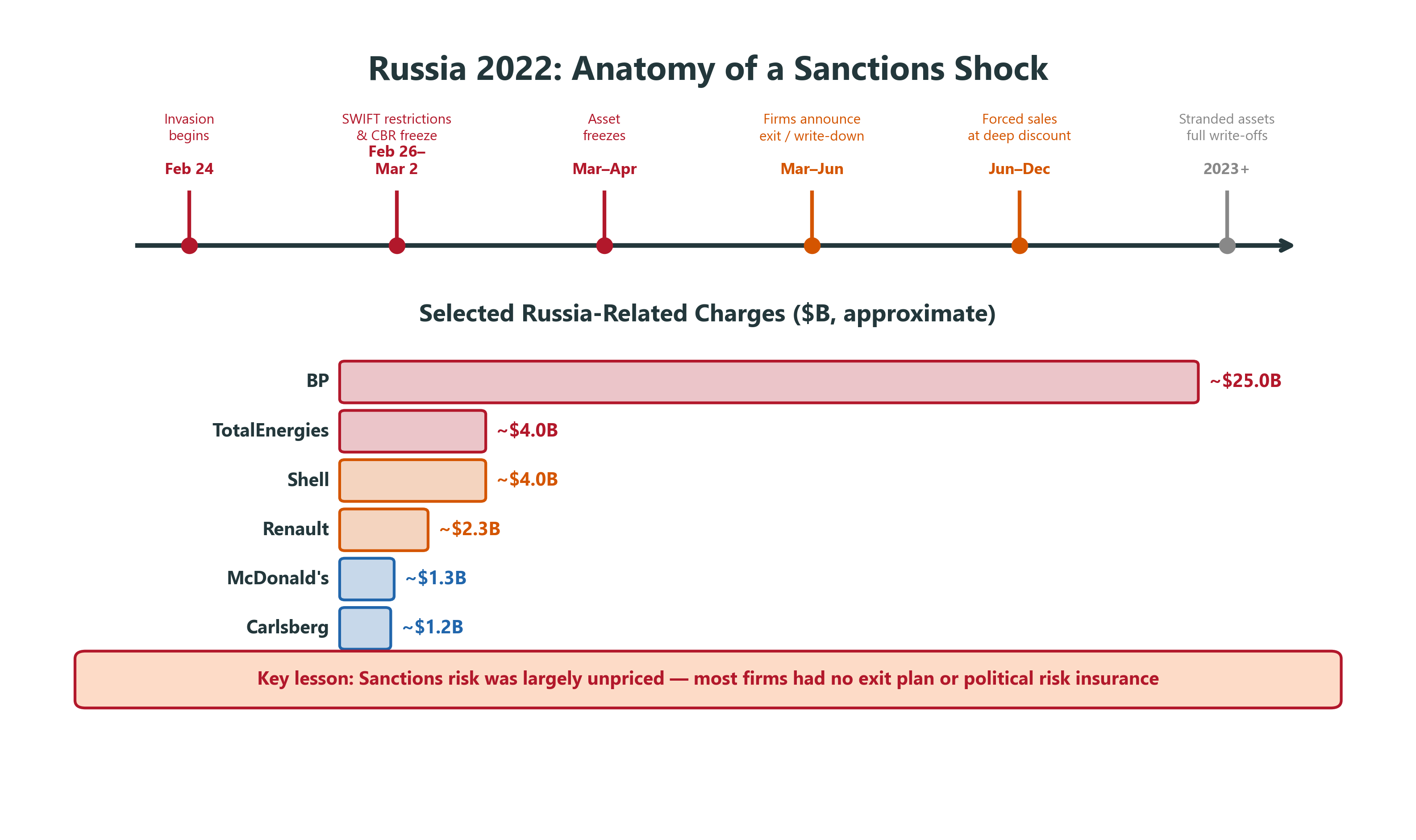
Sanctions as Country Risk: Russia 2022

Walk through the timeline. February 24: Russia invades Ukraine. February 26: joint announcement that selected Russian banks would be removed from SWIFT. February 28: major restrictions on the Central Bank of Russia announced. March 2: EU formally adopts the SWIFT ban for certain banks. March through June: Western companies announce exits and write-downs. The scale is staggering: BP wrote down approximately 25 billion dollars on its Rosneft exit. Shell, TotalEnergies, Renault, McDonald’s, Carlsberg — the losses were widespread. The key lesson: sanctions risk was largely unpriced. Most firms had no exit plan, no political risk insurance covering sanctions, and no scenario analysis that contemplated this outcome.

Lessons from Russia 2022

What went wrong:

• Companies treated Russia as a “normal” emerging market
• No political risk insurance covering sanctions (wasn’t available)
• No exit clauses in JV agreements triggered by sanctions
• Concentration risk: BP’s Rosneft stake represented roughly half of its reported oil and gas reserves and about one-third of production

Implications for future investments:

• Scenario analysis must include sanctions as a tail risk
• Maintain exit optionality: avoid irreversible commitments
• Diversify across geopolitical blocs (not just countries)
• Monitor geopolitical indicators, not just economic ones

Current high-risk jurisdictions: Russia, Iran, North Korea, Myanmar, parts of China (Xinjiang, tech sector)

BP is the most striking case. They had a 19.75% stake in Rosneft. At the time of exit, this stake represented roughly half of BP’s reported proved oil and gas reserves and about a third of its production. When sanctions hit, they had to abandon it, writing down approximately 25 billion dollars. No scenario analysis, no insurance, no exit plan. The lesson for students is clear: sanctions risk is real, it can affect major economies (not just small developing countries), and it needs to be explicitly modeled in any cross-border investment analysis.

ESG and Climate as Country Risk

Stranded asset risk:

• Fossil fuel investments in carbon-dependent countries (Saudi Arabia, Nigeria, Indonesia)
• If global transition accelerates, these assets lose value regardless of country stability

Physical climate risk:

• Infrastructure in flood/drought-prone areas (Bangladesh, Vietnam)
• These risks compound over the project’s life

Transition risk: carbon border adjustments (EU CBAM) penalize countries without carbon pricing

Climate risk operates at the country level in ways that traditional country risk analysis doesn’t capture. A coal-fired power plant in Indonesia faces country risk not because of Indonesian politics, but because of global climate policy. The EU’s Carbon Border Adjustment Mechanism means that countries without carbon pricing will face export tariffs, changing their competitive position. These are new forms of country risk that need to be incorporated into cash flow scenarios.

Climate Risk in the CF Framework

Use scenario analysis (Method 2) with climate-specific scenarios:

Scenario	Prob.	Impact on CF
Orderly transition (Paris targets)	30%	Gradual decline after year 5
Delayed transition (sudden policy)	40%	Sharp decline in year 8-10
No transition (business as usual)	20%	CFs stable, physical risks rise
Accelerated transition	10%	Rapid decline from year 3

• TCFD/ISSB frameworks provide standardized scenarios
• Climate risk is back-loaded (10+ years) — DR adjustment even less appropriate
• Discount rate doesn’t change — these are CF adjustments

Climate risk is a perfect use case for scenario analysis. The key insight is that climate risk is time-varying and back-loaded: most of the impact comes in years 5-15 of a project’s life. This makes the DR adjustment approach even more inappropriate, because the compounding effect of a higher discount rate would crush these later cash flows disproportionately. Using CF adjustment with time-varying scenarios is much more appropriate.

BEPS Pillar Two: Global Minimum Tax

OECD/G20 agreement (effective 2024+): 15% minimum effective tax rate for large MNE groups

• Applies to MNE groups with consolidated revenue > €750M (smaller firms are out of scope)
• If a subsidiary’s effective rate < 15%, a top-up tax is collected
  • Often by the parent country, but many jurisdictions have adopted a qualified domestic minimum top-up tax (QDMTT), collecting the top-up themselves

Impact on country risk analysis:

• Ireland: statutory rate remains 12.5% for out-of-scope firms; in-scope MNE groups face the 15% framework
• Singapore: introduced a domestic top-up tax to retain revenue that would otherwise flow to parent countries
• Tax shields from low-tax subsidiaries may shrink for large MNEs (affects APV Step 2)

Connection to valuation:

• For in-scope firms, reduces the benefit of tax-driven location choices
• Country attractiveness shifts toward real factors (infrastructure, talent, supply chains)

BEPS Pillar Two is a fundamental change in international tax, but the details matter. It only applies to large MNE groups above the €750M revenue threshold — smaller firms are unaffected. The top-up tax mechanism is more nuanced than “the parent country collects”: many countries have adopted QDMTTs, which let them collect the top-up domestically rather than ceding revenue to the parent jurisdiction. Ireland’s 12.5% statutory rate still applies to firms below the threshold or outside the scope, while in-scope groups effectively face 15%. Singapore similarly introduced a domestic top-up rather than simply losing competitiveness. For valuation, the key implication is that tax shields in Step 2 of APV may be smaller for large MNEs in formerly low-tax jurisdictions. Country competitiveness increasingly depends on real factors, not headline tax rates.

Part 6: Putting It All Together

Let’s put everything together with a comprehensive worked example and then summarize the complete cross-border valuation toolkit.

Worked Example: Vietnam Manufacturing Plant

A US firm is evaluating a $50M manufacturing plant in Vietnam

Parameter	Value
Expected annual CF (base case)	$12M for 10 years
Vietnamese sovereign spread	2.5%
ICAPM discount rate (from L11)	11%
MIGA insurance premium	1.2% of insured value p.a.
Insured value	$50M (book value of plant)

Here’s our worked example. A US firm is considering a 50 million dollar manufacturing plant in Vietnam. Vietnam has a moderate sovereign spread of 2.5%, reflecting its status as a stable but developing economy. The ICAPM discount rate from Lecture 11’s framework is 11%. MIGA offers political risk insurance at 1.2% of the 50 million book value per year, covering expropriation, currency inconvertibility, and war/civil disturbance.

Step 1: The Wrong Way (DR Adjustment)

Add sovereign spread to discount rate:

\[r_{adjusted} = 11\% + 2.5\% = 13.5\%\]

\[\text{NPV} = -50 + \sum_{t=1}^{10} \frac{12}{(1.135)^t} = -50 + 63.8 = \$13.8\text{M}\]

• Simple but wrong for all five reasons discussed
• Useful as a benchmark, but conceptually flawed

The naive approach gives an NPV of 13.8 million. We know this is wrong because it double-counts risk, treats all projects equally, confuses systematic and idiosyncratic risk, ignores deal structure, and includes the full risk premium from the spread as if it were expected loss. But it’s a useful benchmark to compare against the correct approaches.

Step 2: CF Adjustment (Bond-Implied)

Default probability from spread: \(p = \frac{0.025}{0.95} \approx 2.6\%\)/year

\[\text{NPV} = -50 + \sum_{t=1}^{10} \frac{12 \times (1-0.026)^t}{(1.11)^t} = -50 + 62.6 = \$12.6\text{M}\]

• Gives a similar NPV to the DR method ($12.6M vs $13.8M)
• With consistent risk-neutral assumptions, DR and CF methods are mathematically close
• The advantage of CF adjustment is conceptual flexibility, not necessarily a different number

Using the CF adjustment with a bond-implied default probability of 2.6% gives an NPV of 12.6 million, actually slightly below the DR method. This is expected: the bond-implied formula p = spread/(1-recovery) gives a risk-neutral probability that, when applied to the CF method, produces a result close to (and in this case slightly below) the DR method. The key advantage of the CF approach is not that it always gives a higher value — it’s that it allows project-specific adjustment, partial-loss scenarios, and time-varying risk. The DR method locks you into a single, uniform penalty.

Step 3: APV with Insurance (Preferred)

Uninsured NPV (no country risk):

\[\text{NPV}_{uninsured} = -50 + \sum_{t=1}^{10} \frac{12}{(1.11)^t} = -50 + 70.7 = \$20.7\text{M}\]

Insurance cost: MIGA premium = 1.2% \(\times\) $50M = $0.6M/year

\[\text{PV(premiums)} = \sum_{t=1}^{10} \frac{0.6}{(1.11)^t} = \$3.5\text{M}\]

Insured NPV:

\[\text{NPV} = 20.7 - 3.5 = \$17.1\text{M}\]

The APV approach gives the highest NPV at 17.1 million. Step 1: value the project ignoring country risk, giving 20.7 million. Step 2: subtract the PV of insurance premiums at 3.5 million. The result is 17.1 million. This is substantially higher than both the DR method (13.8M) and the bond-implied CF method (12.6M). The difference comes because the insurance premium of 1.2% reflects a market-priced, deal-specific assessment of the insurable country risk, which is much less than the full sovereign spread of 2.5%. The spread includes a risk premium and covers risks beyond what is relevant to this specific project.

Comparing All Three Methods

Method	NPV	Comment
DR adjustment (wrong)	$13.8M	Conceptually flawed, inflexible
CF adjustment (bond-implied)	$12.6M	Consistent estimate, but binary
APV with insurance (preferred)	$17.1M	Market-priced, deal-specific

• Difference: $3.3M between DR and APV approach (19% gap)
• DR and CF methods give similar results when derived from the same spread
• The APV method is substantially higher because the insurance premium reflects deal-specific risk, not the full sovereign spread

In practice, supplement Method 3 with scenario analysis for uninsurable risks (sanctions, climate, regulatory changes)

The key comparison is between the DR method (13.8M) and the APV method (17.1M). The gap of 3.3 million, or 19%, is substantial for a 50M investment. The CF method at 12.6M gives a similar result to the DR method because both use the same sovereign spread as their starting point. The APV method is higher because the MIGA insurance premium (1.2%) is a deal-specific, market-priced measure of insurable risk — much lower than the full sovereign spread (2.5%), which includes a risk premium and risks not relevant to this project. The recommendation is to use APV as the primary method and supplement with scenario analysis for risks that insurance doesn’t cover.

The Complete Cross-Border Valuation Toolkit

Step	Component	Lecture
1	Base-case NPV (all-equity, no country risk)	L10 (APV)
	\(\hookrightarrow\) Discount rate	L11 (ICAPM)
	\(\hookrightarrow\) Cash flows in domestic currency	L11 (returns)
2	+ Tax shields	L10 (APV Step 2)
3	+ Financing side effects (subsidies, guarantees)	L10 (APV Step 3)
4	– Country risk adjustment	L12 (this lecture)
	\(\hookrightarrow\) CF adjustment or APV with insurance

This slide shows the complete toolkit. Step 1 comes from Lecture 10’s APV framework, with the discount rate from Lecture 11’s ICAPM. Steps 2 and 3 are from Lecture 10 (tax shields and financing side effects). Step 4 is from this lecture: country risk adjustment using CF methods, not DR methods. Together, these three lectures give students a complete framework for valuing any cross-border investment.

Course Connections

• L3 (PPP) \(\rightarrow\) determines if FX risk is real
• L5 (UIP / carry) \(\rightarrow\) is there an FX risk premium?
• L6–8 (hedging) \(\rightarrow\) can you hedge FX risk? At what cost?
• L10 (APV) \(\rightarrow\) valuation structure
• L11 (ICAPM) \(\rightarrow\) discount rate
• L12 (country risk) \(\rightarrow\) cash flow adjustment

The arc: exchange rates \(\rightarrow\) hedging \(\rightarrow\) valuation \(\rightarrow\) discount rate \(\rightarrow\) country risk = complete framework for international corporate finance

This lecture completes the major arc of the course. We started with understanding exchange rates (PPP, UIP), learned how to hedge them, then built a valuation framework (APV), determined the right discount rate (ICAPM), and now handled country risk. Every piece connects to the others. PPP determines whether FX risk is real (which matters for the ICAPM). UIP determines whether carry trades work (which matters for factor models). Hedging determines whether FX beta is zero (which simplifies the ICAPM). And all of it feeds into the APV framework.

Key Takeaways

1. Country risk is an umbrella for correlated risks: transfer, sovereign, political, currency, and sanctions

2. Never add a sovereign spread to the discount rate (the 500bp fallacy)
   • Double-counts, ignores deal structure, biases against long-lived projects

3. Adjust cash flows, not the discount rate
   • Bond-implied probability for quick estimates
   • Scenario analysis for complex, multi-risk settings
   • APV with insurance as the preferred approach

4. Modern risks require updating the classical framework
   • Sanctions (Russia 2022), climate/ESG, BEPS Pillar Two

Four key takeaways. First, country risk is not a single thing but a bundle of correlated risks. Second, the most common practice (adding spread to WACC) is fundamentally wrong for at least five reasons. Third, the right approach is to adjust expected cash flows using one of three methods, with APV plus insurance being preferred. Fourth, the classical framework needs updating to account for sanctions, climate risk, and global tax reform. These are the concepts students should take away from this lecture.