International Finance

International Cost of Capital: ICAPM and Currency Risk Factors

Main Issues

• Why does international asset pricing differ from domestic?
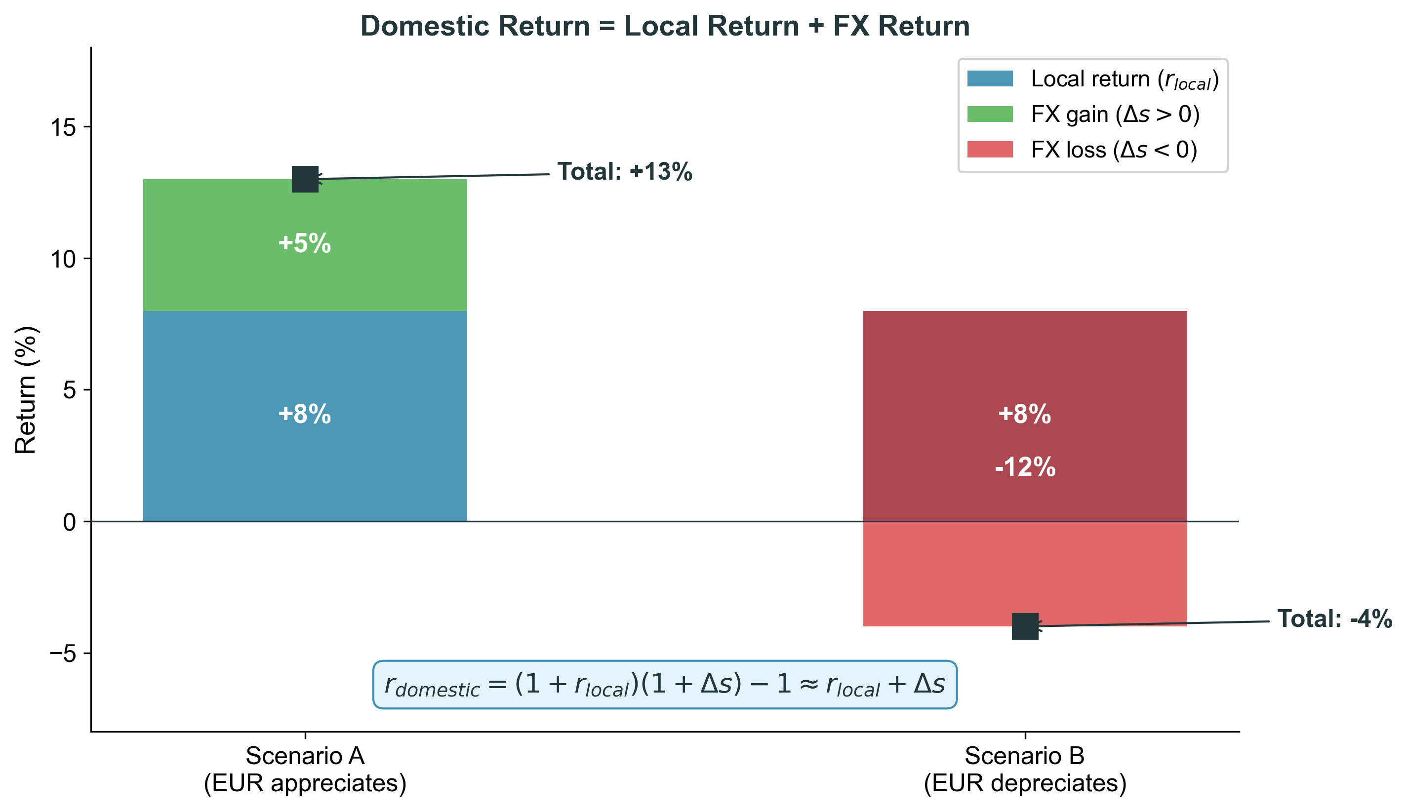
• Computing returns across currencies: the domestic investor’s perspective
• The CAPM and the tangency portfolio argument

• Why CAPM breaks internationally: which market portfolio? FX risk?
• The 2×2 ICAPM framework with worked examples
• Currency risk factors: carry, dollar, momentum, volatility

• Connection: this gives us the discount rate for APV Step 1 (Lecture 10)

This lecture answers the question Lecture 10 left open: “What discount rate should we use for the base case in APV?” We build from the domestic CAPM, show why it breaks internationally, develop the ICAPM, and then move to modern currency factor models for practical implementation.

Why International Asset Pricing?

The Open Question from Lecture 10

• Lecture 10: APV framework for cross-border valuation

• Step 1 requires the unlevered cost of equity: \(r_{project}\)
• We left this open — now we answer it

• The challenge: international projects face risks that don’t arise domestically
  • Which market portfolio should we use? US? World? Local?
  • Does exchange rate risk carry a separate premium?

Lecture 10 established the five-step APV framework. Step 1 — the branch stage — discounts operating cash flows at the unlevered cost of equity. But we never said how to compute that rate. This lecture fills that gap. The next lecture (Country Risk) fills in APV Step 4.

Two Problems with Going International

Problem 1: Which market portfolio?

• A US firm evaluating a project in India:
  • Use the S&P 500? The BSE Sensex? MSCI World?
  • The answer depends on financial market integration

Problem 2: Exchange rate risk

• Is FX risk separately priced, or is it already captured in the market factor?
• The answer depends on product market integration (PPP)

These are not just theoretical — they give different discount rates

These two questions structure the entire lecture. Problem 1 is about the market portfolio (financial integration). Problem 2 is about whether we need a second factor for FX risk (product market integration / PPP). The 2x2 framework later combines these two dimensions.

International Diversification and Home Bias

• Cross-country equity correlations are lower than within-country
  • Diversification benefits are real and well-documented

• Yet investors hold 70–80% domestic equity (the “home bias puzzle”)
  • Information asymmetries, familiarity bias, institutional constraints
  • Hedging domestic consumption risk (if PPP fails)

• This puzzle matters for asset pricing:
  • If investors are home-biased, is the world CAPM the right model?
  • If they should hold global portfolios, domestic CAPM is wrong

We keep this brief — just enough to motivate why the choice of market portfolio matters. The home bias puzzle has been documented since French and Poterba (1991). Despite some decline over time, home bias remains large, especially in emerging markets.

Returns in International Markets

Computing Returns in Domestic Currency

A US investor buying German stocks earns two components (HC \(=\) USD, FC \(=\) EUR):

1. Local return (\(r_{local}\)): the DAX return in EUR.
2. FX return (\(x\)): the percentage change in \(S^{USD/EUR}\), the USD price of one EUR. ;That is, \(x = S_1/S_0 - 1\).

Exact formula: \[r_{domestic} \;=\; (1 + r_{local})(1 + x) - 1\]

Approximation (for small returns): \[r_{domestic} \;\approx\; r_{local} + x\]

Key principle: We always evaluate returns from the perspective of the domestic investor

This is foundational. Everything that follows — CAPM, ICAPM, factor models — is about pricing assets in domestic currency terms. The cross-product term is usually small but can matter for high-volatility emerging market currencies.

Domestic return decomposition: approximate

Approximation: \(r_{dom} \approx r_{local} + x\). Exact: \((1+r_{local})(1+x) - 1\). Exact totals: A \(= 13.4\%\), B \(= -5.0\%\).

Scenario A: DAX returns 8%, EUR appreciates 5% against USD. Additive approximation: 13%; exact: 13.4%. Scenario B: same DAX return, EUR depreciates 12%. Additive: -4%; exact: about -5.0%. The chart labels use the additive approximation because it is the pedagogically clean teaching object; the cross-product term matters once returns or FX moves are large.

Variance of Domestic Returns

The variance of the domestic return has three components:

\[\mathrm{Var}(r_{dom}) \;=\; \mathrm{Var}(r_{local}) \;+\; \mathrm{Var}(x) \;+\; 2\,\mathrm{Cov}(r_{local},\, x)\]

Key implication: Even a risk-free foreign bond is risky to a domestic investor!

• German 1-year T-bill: riskless for a German investor.
• For a US investor: \(\mathrm{Var}(r_{dom}) = 0 + \mathrm{Var}(x) + 0 = \mathrm{Var}(x)\).
• \(S^{USD/EUR}\) can move 10–15% per year — far from riskless!

Unless PPP holds perfectly (which it doesn’t — Lecture 3)

This is why exchange rate risk must enter asset pricing. Different investors see different risk profiles for the same asset. A British investor sees the US T-bill as risky (GBP/USD fluctuates), while a US investor sees it as risk-free. This violates the homogeneous expectations assumption of the standard CAPM.

Why This Matters for Asset Pricing

• Investors in different countries see different real risk–return profiles for the same asset when PPP fails.

• This breaks the CAPM’s homogeneous-expectations / common-investment-opportunity-set assumption: investors evaluate real payoffs in different consumption baskets.

• We need a model that accounts for this heterogeneity.

Two ingredients needed:

1. Financial market integration: which market portfolio?
2. Product market integration / PPP: is FX risk separately priced?

The mechanism behind the heterogeneity is real returns measured in different consumption baskets. Once PPP holds, all investors agree on real returns and the CAPM homogeneity assumption is restored. This is the reason PPP failure – not just nominal FX volatility – is what makes FX a separately priced risk.

The Domestic CAPM

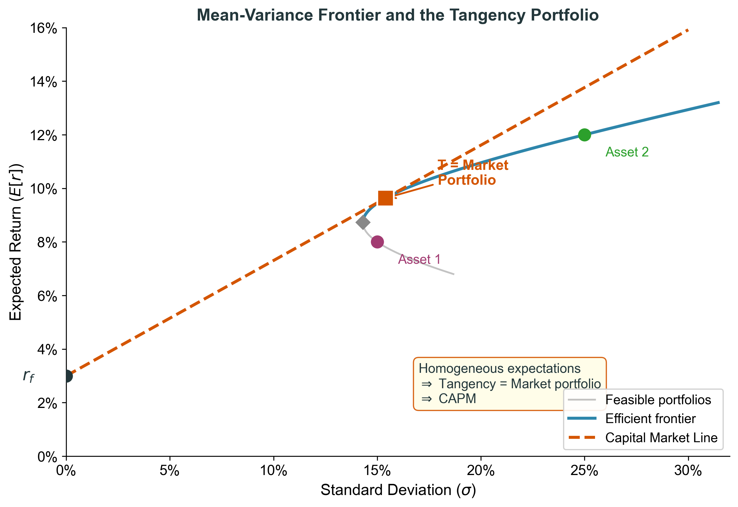
Mean-Variance Optimization

The efficient frontier shows the set of portfolios that maximize expected return for a given level of risk. Adding the risk-free asset creates the Capital Market Line. Every investor holds a combination of the risk-free asset and the tangency portfolio. Under homogeneous expectations, all investors agree on the tangency portfolio, so in equilibrium it must equal the market portfolio.

Tangency Portfolio = Market Portfolio

Homogeneous opportunities: all investors face the same assets and risk-free rate

Homogeneous expectations: all investors agree on means, variances, covariances

\(\Rightarrow\) Everyone holds the same tangency portfolio as their risky allocation

Equilibrium: demand = supply

\(\Rightarrow\) Tangency portfolio (demanded) = Market portfolio (supplied)

This is the key insight of the CAPM: in equilibrium, the market portfolio is the tangency portfolio

These assumptions are strong. Internationally, they’re even harder to justify because investors in different countries face different risk-free rates and see different returns on the same assets (in their own currency). That’s where the CAPM breaks.

The CAPM Equation

Risk is measured relative to the market portfolio:

\[\beta_j = \frac{\text{Cov}({\widetilde{r}}_j, {\widetilde{r}}_M)}{\text{Var}({\widetilde{r}}_M)}\]

The CAPM:

\[E[{\widetilde{r}}_j] = r_f + \beta_j \times \underset{\color{#2E86AB}{\small\textbf{market risk premium}}}{\bbox[#dbeafe,5px,border:1px solid #2E86AB]{\;(E[{\widetilde{r}}_M] - r_f)\;}}\]

• \(\beta = 0\): earn the risk-free rate (no systematic risk)
• \(\beta = 1\): earn the market return
• \(\beta > 1\): amplified market risk, higher expected return

The CAPM says that only systematic risk (beta) is priced. Idiosyncratic risk can be diversified away. This is the workhorse model for cost of capital estimation domestically. Beta services (Bloomberg, MSCI) provide estimates for industries and firms.

CAPM: Numerical Examples

Suppose the market premium is 5% and \(r_f = 2\%\):

\(\beta\)	Expected Return	Interpretation
0	2%	Risk-free rate
1	7%	Market return
2	12%	Aggressive (amplified risk)
\(-0.5\)	\(-0.5\%\)	Hedge asset (insurance)

• In practice: beta services provide estimates for industries/firms
• But they typically assume the CAPM holds country-by-country with the domestic market
• Is this the right benchmark? \(\rightarrow\) Not always!

The negative beta case is interesting — it means the asset moves opposite to the market, so it acts as insurance. Investors are willing to accept negative expected returns for this hedge property. Gold and some currencies can have negative betas in certain periods.

Why CAPM Breaks Internationally

Problem 1: Financial Integration

A country is financially integrated if:

• Firms borrow and raise funds in international capital markets
• Investors directly invest across borders
• Cross-border capital flows are substantial

If integrated (US, UK, Germany, Japan): benchmark = world market portfolio

If segmented (some EM with capital controls): benchmark = domestic market portfolio

Practical proxy for world market: a low-cost global equity ETF such as the Vanguard Total World Stock ETF (VT), which tracks the FTSE Global All Cap Index.

Financial integration means that assets are priced by global investors, not just local ones. In an integrated market, a stock’s expected return depends on its covariance with the world market, not the local market. Most developed markets are integrated; many emerging markets are partially or fully segmented.

Venus and Mars: Segmented Markets

Imagine two planets with the same currency (no FX risk for now):

Parameter	Mars	Venus
Risk-free rate	5%	5%
Market volatility	30%	30%
Risk aversion (\(\gamma\))	0.45	0.65

Expected returns on domestic markets:

\[\mu_M = 5\% + 0.45 \times 0.30^2 = 9.05\%\] \[\mu_V = 5\% + 0.65 \times 0.30^2 = 10.85\%\]

Sharpe ratios: 0.135 (Mars) vs. 0.195 (Venus)

This example, from the old lecture slides, is pedagogically powerful because it removes FX risk entirely. The only question is: does financial integration matter? Same assets, same volatility, but different risk aversion leads to different prices and expected returns.

Segmented: Cost of Capital Differs!

A project on Venus with \(\beta = 0.75\):

Venus investor (uses Venus market, premium = 5.85%):

\[E[r] = 5\% + 0.75 \times 5.85\% = 9.39\%\]

Mars investor (uses Mars market, premium = 4.05%):

\[E[r] = 5\% + 0.75 \times 4.05\% = 8.04\%\]

Same project, same beta, DIFFERENT cost of capital!

\(\Rightarrow\) When markets are segmented, who you are matters

This is the key insight. Under segmentation, the same project has a different cost of capital depending on who is valuing it. The Mars investor would accept a lower return because Mars is less risk-averse. This means an investment could be profitable for a Mars firm but not for a Venus firm — purely because of where the investor is based.

Integrated: Cost of Capital Is the Same

Now open the border — markets are financially integrated:

Parameter	Integrated World
Aggregate risk aversion (\(\gamma\))	0.53
World market return	7.38%
World market volatility	21.21%

Same project on Venus, \(\beta = 0.75\):

\[E[r] = 5\% + 0.75 \times 2.38\% = 6.79\%\]

\(\Rightarrow\) Same for both investors! Who you are doesn’t matter. Only systematic risk (relative to the world) is priced.

Integration lowers the cost of capital (6.79% vs 8-9%) because diversification across planets reduces the effective risk. The world portfolio has lower volatility (21.21% vs 30%) due to imperfect correlation. This is the core argument for financial globalization reducing the cost of capital in emerging markets.

Problem 2: Exchange Rate Risk

Now add different currencies. Ignore FX risk?

If PPP holds. Nominal FX movements are offset by relative price changes. Real returns are unaffected by exchange-rate movements, so nominal FX risk is not separately priced. Use a single-factor CAPM with the appropriate market portfolio.

If PPP fails. Investors in different countries see different real returns on the same asset, because the relevant consumption basket differs. The standard CAPM assumptions break down and an FX factor may be needed.

\(\Rightarrow\) PPP failure is what makes FX a separately priced risk factor.

This is where Lecture 3 (PPP) feeds in. We showed that PPP fails dramatically in the short and medium run. Large and persistent deviations from PPP mean that real exchange rate risk is substantial. This is the second dimension of the 2x2 framework.

Convention reminder: notation

Throughout the lecture:

• \(r \;=\;\) home-currency risk-free rate.
• \(r^* \;=\;\) foreign-currency risk-free rate.
• \(s \;=\; \log S\), the (log) exchange rate quoted HC/FC (home-currency price of one unit of foreign currency).

\(\Delta s > 0\) means the foreign currency appreciates from the home investor’s perspective.

The excess return on a foreign risk-free investment for the home investor is \[E[\Delta s] \;+\; r^* \;-\; r.\] Under UIP, \(E[\Delta s] + r^* - r = 0\). Under failed UIP, this is the FX risk premium that enters the ICAPM formulas below.

Bridge: in the return-decomposition slides, \(x = S_1/S_0 - 1\) was the simple FX return. In the ICAPM, \(s = \log S\) so \(\Delta s\) is the log FX return. For small changes, \(\Delta s \approx x\).

Convention check before formula: HC per FC means a higher \(s\) is a stronger foreign currency. The bracket \(E[\Delta s] + r^* - r\) is the same expression that appeared in Lectures 4 and 5 (CIP/UIP). We use \(r\) and \(r^*\) consistently from here on.

The Two-Factor International CAPM

When PPP fails and financial markets are integrated:

\[E[\widetilde{r}_j - r] = \underset{\color{#2E86AB}{\small\textbf{world market risk}}}{\bbox[#dbeafe,5px,border:1px solid #2E86AB]{\;\beta_W \,(E[\widetilde{r}_W] - r)\;}} \;+\; \underset{\color{#D45500}{\small\textbf{exchange rate risk}}}{\bbox[#fce7d6,5px,border:1px solid #D45500]{\;\beta_s \,(E[\Delta\widetilde{s}] + r^* - r)\;}}\]

\(\beta_W\) and \(\beta_s\) are multivariate regression coefficients, estimated jointly from \[\widetilde{r}_j - r \;=\; \alpha \;+\; \beta_W\,(\widetilde{r}_W - r) \;+\; \beta_s\,\bigl(\Delta\widetilde{s} + r^* - r\bigr) \;+\; \widetilde{\varepsilon}_j.\]

The simple covariance-ratio formula \(\beta = \mathrm{Cov}/\mathrm{Var}\) applies only in the single-factor case, or when the two factors are orthogonal.

\(\Rightarrow\) Two sources of systematic risk, two risk premia.

This is the Adler-Dumas (1983) International CAPM with one bilateral exchange rate. The next slide generalizes to N currencies. The factor-model section later in the lecture handles the multi-currency case in practice.

From one foreign currency to many

For a multinational with exposure to \(N\) currencies, the bilateral ICAPM generalizes to

\[E[\widetilde{r}_j - r] \;=\; \beta_W \,(E[\widetilde{r}_W] - r) \;+\; \sum_{k=1}^{N} \beta_{s,k}\,\bigl(E[\Delta\widetilde{s}_k] + r^*_k - r\bigr),\]

where:

• \(s_k\) is the (log) HC price of currency \(k\),
• \(r^*_k\) is the risk-free rate in currency \(k\),
• \(\beta_{s,k}\) is the exposure to currency \(k\).

The \(\beta_{s,k}\)’s (and \(\beta_W\)) are multivariate exposure coefficients, estimated jointly.

Conceptually clean, but hard to estimate: many currencies, many betas, and the exchange rates are strongly correlated. This motivates currency factor models (later in the lecture).

In principle there is one FX premium per currency. In practice the bilateral betas are noisy and the FX premia co-move strongly. Factor models exploit this co-movement by replacing the N bilateral betas with a small number of factor loadings (DOL, HML carry, momentum, volatility).

The 2×2 ICAPM Framework

Three Key Questions

Before applying the 2×2 framework, consider:

Q1: What if UIP holds (\(E[\Delta\widetilde{s}] + r^* - r = 0\))?

• FX risk premium is zero \(\rightarrow\) \(\beta_s\) drops out; single-factor CAPM suffices

Q2: What if the carry trade is profitable?

• FX risk premium \(\neq 0\) \(\rightarrow\) \(\beta_s\) matters; sign depends on FX correlation

Q3: What if the firm hedges all its currency exposure?

• \(\beta_s = 0\) by construction \(\rightarrow\) FX term drops out
• Another reason hedging can be valuable (Lecture 6)

These three questions come from the video script and are very useful for building intuition. Q1: if UIP holds, there’s no compensation for bearing FX risk, so it doesn’t affect expected returns. Q2: the carry trade’s profitability is evidence that FX risk premia exist — recall Lecture 5 showed b = -0.88 on average. Q3: if the firm hedges, its equity returns are no longer correlated with FX, so beta_s becomes zero.

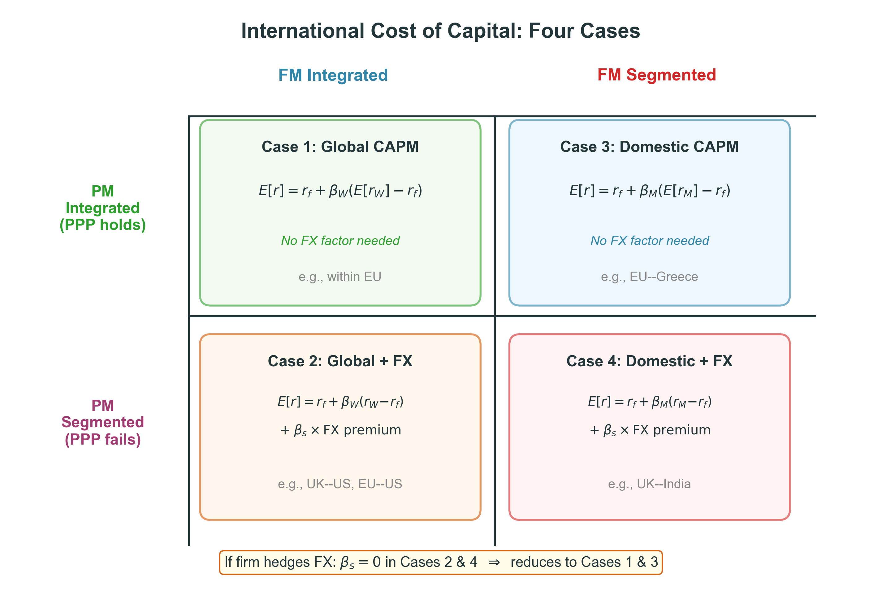
The Four Cases

This is the central organizing framework. The rows represent product market integration (whether PPP holds). The columns represent financial market integration (whether capital flows freely). Each cell gives a different pricing model with different inputs. Most developed-market pairs fall into Case 2 (FM integrated, PM segmented). EM pairs often fall into Case 4.

Case 1: Both Integrated (e.g., within EU)

Product markets integrated (PPP holds) + Financial markets integrated

1. Use your home currency risk-free rate.
2. Use a global index as proxy for the market portfolio.
3. PPP holds: nominal FX movements are offset by relative price changes, so real returns are not affected by exchange-rate movements. No separately priced FX factor is needed.
4. Run a univariate regression to estimate \(\beta_W\).

\[E[\widetilde{r}_j - r] \;=\; \beta_W\,(E[\widetilde{r}_W] - r)\]

This is just the standard CAPM with a global market portfolio.

Case 1 is the simplest case. Within a currency union like the Eurozone, there’s no exchange rate risk and financial markets are highly integrated. The global CAPM applies. Estimate beta against a world index (MSCI World, VT ETF) and use the global equity premium.

Case 2: PM Segmented, FM Integrated (e.g., UK–US)

Product markets segmented (PPP fails) + Financial markets integrated

1. Use your home currency risk-free rate
2. Use a global index as proxy for market portfolio
3. FX risk matters — PPP deviations create real exchange rate risk
4. Run a multivariate regression for \(\beta_W\) and \(\beta_s\)

\[E[\widetilde{r}_j - r] \;=\; \beta_W (E[\widetilde{r}_W] - r) \;+\; \beta_s (E[\Delta\widetilde{s}] + r^* - r)\]

If the company is perfectly hedged: \(\beta_s = 0\) \(\rightarrow\) reduces to Case 1

This is the most common case for developed-market cross-border projects. US-UK, US-Germany, US-Japan — all have integrated financial markets but PPP fails. You need two betas: one for the world market and one for the bilateral exchange rate. Note: if the firm hedges, the FX beta goes to zero and you’re back to the simple global CAPM.

Case 3: PM Integrated, FM Segmented (common-currency/pegged + capital controls)

Product markets integrated (PPP holds) + Financial markets segmented

1. Use your home currency risk-free rate.
2. Use the domestic market portfolio (financial markets are segmented).
3. PPP holds, so nominal FX movements are offset by relative price changes: no separately priced FX factor is needed.
4. This is just the single-country CAPM.

\[E[\widetilde{r}_j - r] \;=\; \beta_M\,(E[\widetilde{r}_M] - r)\]

Back to the textbook domestic CAPM — but with a domestic benchmark.

This case is less common but arises in goods-market-integrated economies with restricted foreign investment, or in common-currency / tightly-pegged regimes that also impose capital controls (e.g., a euro-area sovereign-crisis episode with capital controls). The unifying feature is: prices arbitrage across borders, but capital does not. The domestic market portfolio is then the right benchmark.

Case 4: Both Segmented (e.g., UK–India)

Product markets segmented (PPP fails) + Financial markets segmented

1. Use your home currency risk-free rate
2. Use the domestic market portfolio (capital markets segmented)
3. FX risk matters — PPP deviations plus limited hedging options
4. Run a multivariate regression for \(\beta_M\) and \(\beta_s\)

\[E[\widetilde{r}_j - r] \;=\; \beta_M (E[\widetilde{r}_M] - r) \;+\; \beta_s (E[\Delta\widetilde{s}] + r^* - r)\]

If the company is perfectly hedged: \(\beta_s = 0\) \(\rightarrow\) reduces to Case 3

This is the most complex case. Both product and financial markets are segmented. You need the domestic market beta (not global, because capital can’t flow freely) and the FX beta. Many emerging market pairs fall here: UK investing in India, EU investing in Latin America. Note I’m illustrating with just one exchange rate; in principle there should be one for each relevant currency.

Worked Example: Data

Country A investor valuing a project in Country B. Financial markets are segmented.

Quantity	Symbol	Value
Risk-free rate, Country A	\(r_A\)	3%
Risk-free rate, Country B	\(r_B\)	5%
E[return on A market]	\(E[\widetilde{r}_A]\)	10%
E[return on world market]	\(E[\widetilde{r}_W]\)	8%
E[exchange-rate change]	\(E[\Delta\widetilde{s}]\)	1%
Var(A market)	\(\mathrm{Var}(\widetilde{r}_A)\)	0.0324
Cov(project, A market)	\(\mathrm{Cov}(\widetilde{r}_j, \widetilde{r}_A)\)	0.0432
Cov(project, \(\Delta s\))	\(\mathrm{Cov}(\widetilde{r}_j, \Delta\widetilde{s})\)	0.004
Var(\(\Delta s\))	\(\mathrm{Var}(\Delta\widetilde{s})\)	0.02

This is adapted from the old slides. The student needs to first determine which case applies, then compute the correct cost of capital. Financial markets are given as segmented. The question is: are product markets integrated or segmented?

Testing Product Market Integration

We estimate a PPP regression:

\[\log\!\left(\frac{S_{t+1}}{S_t}\right) \;=\; -0.06 \;+\; 0.89\,\bigl(\pi^A_{t,t+1} - \pi^B_{t,t+1}\bigr).\]

• The slope coefficient (0.89) is not significantly different from 1.
• The constant (\(-0.06\)) is not significantly different from 0.
• \(\Rightarrow\) Cannot reject Relative PPP.

Stylized decision rule for this example. Because the PPP regression does not reject relative PPP, we classify product markets as integrated here.

Financial markets segmented + Product markets integrated \(=\) Case 3.

This is a key empirical step. To apply the 2x2 framework, you need to determine which case applies. Here we test PPP using the relative PPP regression. If the slope is close to 1 and the intercept close to 0, PPP holds and product markets are integrated. In this example, we cannot reject PPP, so we’re in Case 3.

Worked Example: Solution

Case 3: Domestic CAPM (FM segmented, PM integrated). Here \(r_A\) is the home risk-free rate and \(r_B\) is the foreign risk-free rate.

Step 1 — beta:

\[\beta_A \;=\; \frac{\mathrm{Cov}(\widetilde{r}_j,\, \widetilde{r}_A)}{\mathrm{Var}(\widetilde{r}_A)} \;=\; \frac{0.0432}{0.0324} \;=\; 1.333.\]

Step 2 — market premium:

\[E[\widetilde{r}_A] - r_A \;=\; 10\% - 3\% \;=\; 7\%.\]

Step 3 — cost of capital:

\[E[r_j] \;=\; r_A + \beta_A\,(E[\widetilde{r}_A] - r_A) \;=\; 3\% + 1.333 \times 7\% \;=\; \mathbf{12.33\%}.\]

We use the domestic market premium, not the world premium, because financial markets are segmented.

The FX variables in the data table are included so we can also compute the alternative cases in class. Because the PPP test classifies product markets as integrated, the baseline solution reduces to Case 3 and the FX term drops out.

What if PPP failed?

If we instead concluded that PPP fails (Case 4), the FX term enters:

\[\beta_s \;=\; \frac{\mathrm{Cov}(\widetilde{r}_j,\, \Delta\widetilde{s})}{\mathrm{Var}(\Delta\widetilde{s})} \;=\; \frac{0.004}{0.02} \;=\; 0.20.\]

\[\text{FX premium} \;=\; E[\Delta\widetilde{s}] + r_B - r_A \;=\; 1\% + 5\% - 3\% \;=\; 3\%.\]

\[\text{FX add-on} \;=\; 0.20 \times 3\% \;=\; 0.60\%.\]

\[\text{Case 4 cost} \;=\; 12.33\% + 0.60\% \;=\; 12.93\%.\]

Because the baseline PPP test classifies product markets as integrated, the Case 3 solution drops this FX term.

This extension lets students see how Case 4 differs from Case 3 numerically. The data table on the previous slide kept the FX variables precisely so we can run this extension live. The increment is small here only because beta_s is small; with a higher beta_s or a larger FX risk premium the gap would be material.

This is the punch line. Because financial markets are segmented, the relevant benchmark is the domestic market, not the world market. The investor’s own shareholders are the ones who need to be compensated, and they can only diversify domestically. If we had incorrectly used the world market (Case 1), we would have gotten a different answer.

Currency Risk Factors

The Practical Problem with Bilateral Betas

The 2×2 framework uses \(\beta_s\) for one bilateral exchange rate

But a multinational faces MANY currencies:

• A European firm with subsidiaries in the US, Japan, UK, Brazil…
• Cannot reliably estimate \(N\) separate bilateral betas

Solution: Factor models

• Identify common risk factors in currency markets
• Just as Fama-French replaced single-beta CAPM in equities
• A firm’s currency exposure can be decomposed into factor loadings

\(\Rightarrow\) From bilateral \(\beta_s\) to systematic factor exposures

This is the transition from theory to practice. The 2x2 framework is theoretically elegant but practically limited when firms face many currencies. Factor models solve this by identifying the common sources of risk that drive currency returns. This parallels the move from the CAPM to multi-factor models in equities.

From UIP Failure to Risk Factors

Recall from Lecture 5: UIP fails dramatically.

• 75+ studies: average slope \(b = -0.88\) (should be \(+1\)).
• \(\Rightarrow\) FX risk premia exist and are economically large.

UIP failure creates currency excess returns; when PPP also fails, those currency returns affect real payoffs and can enter the cost of capital.

Key insight (Lustig, Roussanov, Verdelhan, RFS 2011): sort currencies by interest rate into portfolios; high-interest-rate currencies earn high average returns \(\rightarrow\) carry factor.

This connects directly to Lecture 5’s empirical findings. UIP failure means there is a risk premium in currency markets. LRV (2011) showed that this risk premium has a cross-sectional structure: it’s not random which currencies earn high or low returns. Sorting by interest rates reveals a systematic pattern, just like sorting by book-to-market reveals value in equities.

The Carry Factor (HML)

Construction: Sort currencies into 6 portfolios by interest rate

• Long highest interest rate portfolio
• Short lowest interest rate portfolio
• The difference is the HML carry factor

Key statistics (LRV 2011):

	Mean Excess Return	Std Dev	Sharpe Ratio
HML Carry	3.31%	9.56%	0.35

• Positive average returns, but with occasional sharp drawdowns.
• Downside risk is an important feature of carry returns.

The carry factor is the most important currency factor. It earns a positive average return because high interest rate currencies tend to appreciate (violating UIP), so you earn both the interest differential and the FX appreciation. But the distribution is highly negatively skewed — the returns come from many small gains and a few very large losses.

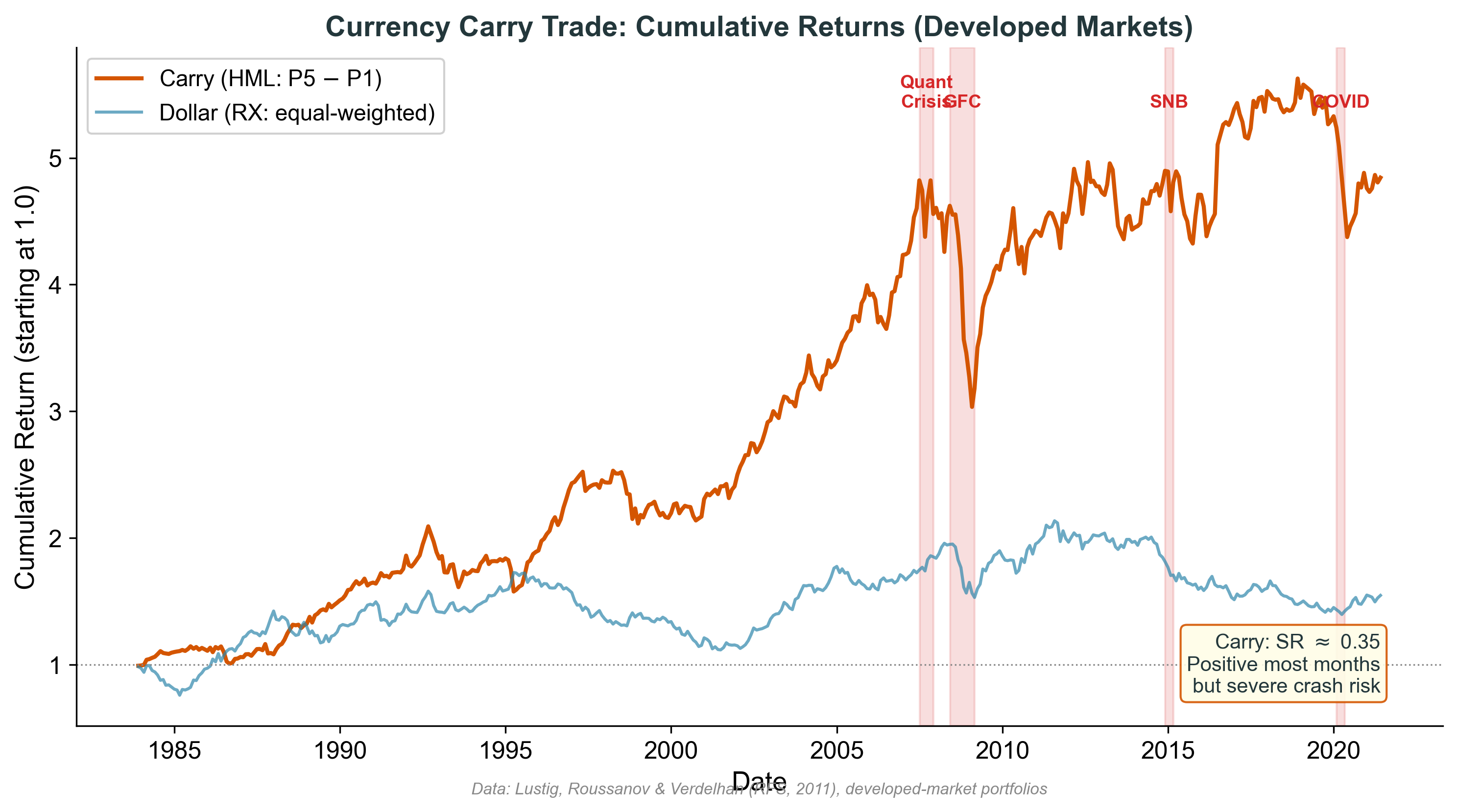
Carry Trade: Cumulative Returns

This figure shows the cumulative return of a G10 carry trade strategy (long high interest rate currencies, short low interest rate currencies). The upward trend is clear, but note the sharp drawdowns during crisis episodes. The GFC in 2008 was particularly devastating as safe-haven currencies (JPY, CHF) surged. The dollar factor (equal-weighted) shows the average return of holding foreign currencies vs USD.

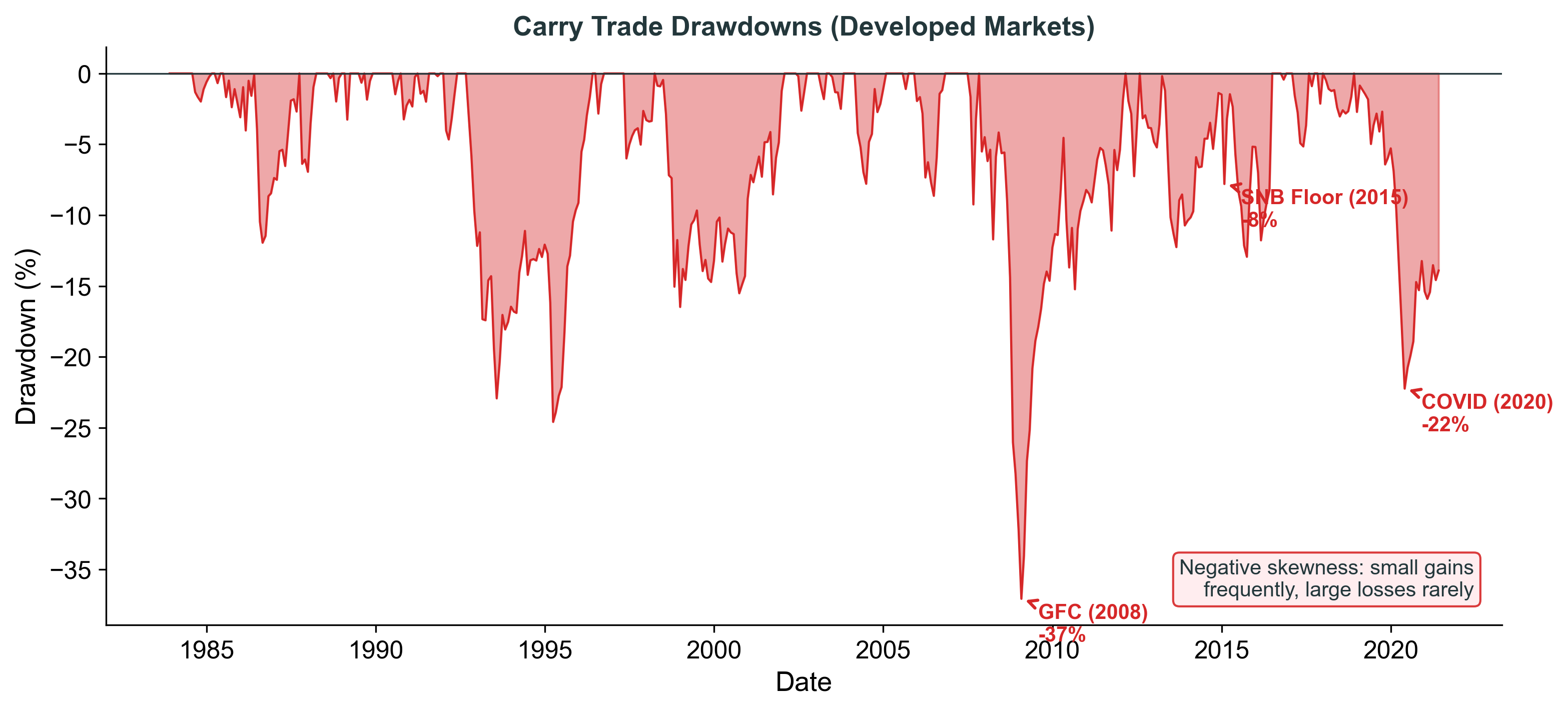
Carry Trade: Crash Risk

The drawdown chart makes the crash risk visceral. Carry trades can lose 20-30% in a few months during crises. This negative skewness is the key risk characteristic. The carry premium is compensation for bearing this crash risk. This connects to Lecture 8’s options content: the carry trade payoff resembles selling put options — you collect small premiums but face large losses in tail events.

The Dollar Factor (DOL)

Average return of all currencies against the USD

• Captures broad dollar strength/weakness
• Acts as the “level” factor (carry is the “slope”)

When global risk appetite falls:

• USD strengthens (flight to safety)
• DOL turns negative; carry also crashes (high-yield currencies fall)

\(\Rightarrow\) DOL and carry are correlated but distinct

• DOL: directional dollar bet
• Carry: cross-sectional bet (long high minus short low)

The dollar factor captures the common component of all currency returns vs USD. It’s related to global risk appetite — when investors are risk-averse, they buy USD and sell risky currencies. DOL can be thought of as a “market factor” for currencies, analogous to the equity market factor.

Momentum and Volatility Factors

Momentum:

• Past currency winners continue to outperform (3-12 month horizon)
• Similar to equity momentum, but in FX
• Sharpe ratio \(\approx\) 0.45 — higher than carry!

Volatility:

• When global FX volatility spikes, carry crashes
• A “volatility innovation” factor captures this
• Negative correlation with carry returns
• Sharpe ratio \(\approx\) 0.30

These factors capture different dimensions of currency risk

Momentum in currencies was documented by Menkhoff et al. (2012). It’s distinct from carry — you can have a high interest rate currency with negative momentum (e.g., after a crisis). The volatility factor captures the idea that carry traders are essentially selling volatility insurance. When volatility spikes, they lose. These factors are not perfectly correlated, so they capture different risk dimensions.

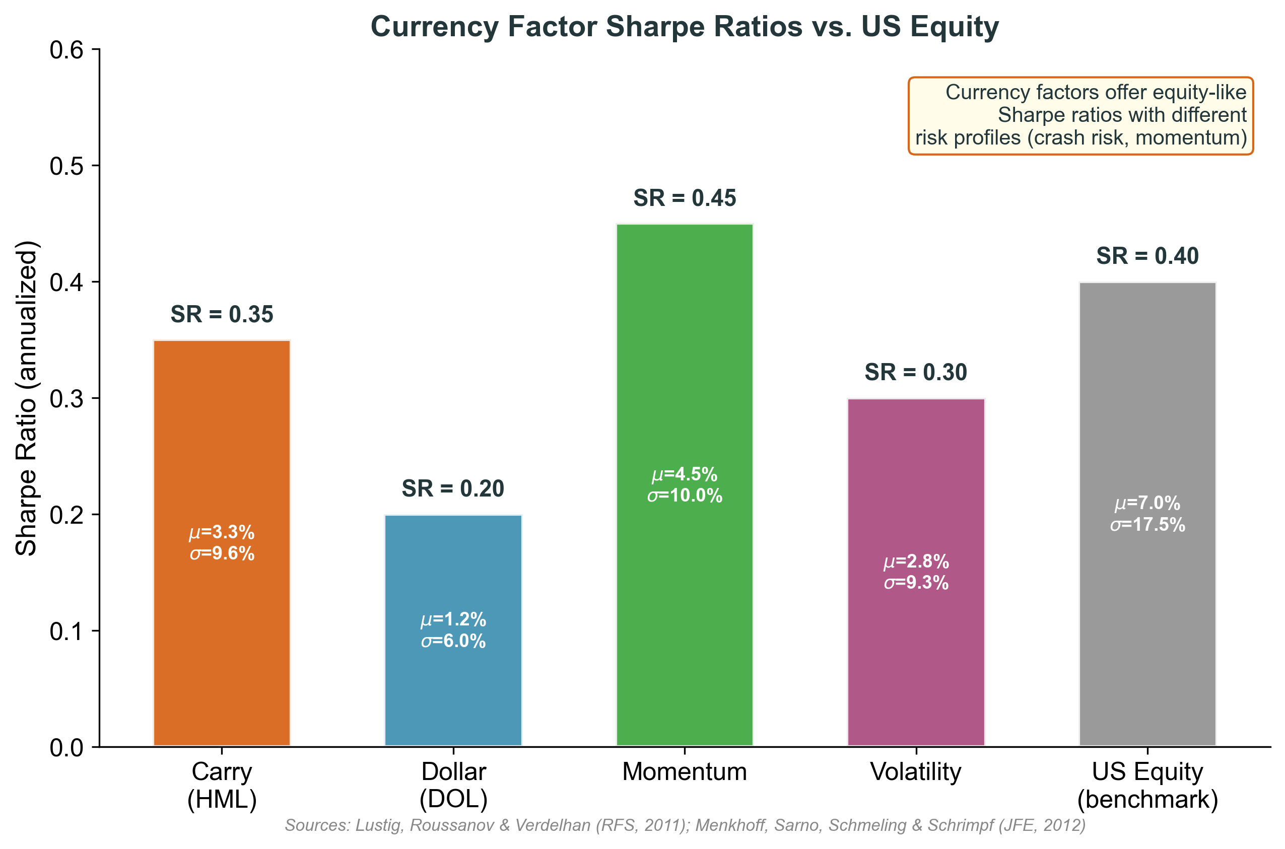
Factor Sharpe Ratio Comparison

This comparison puts currency factors in context. Carry and momentum have Sharpe ratios comparable to or higher than US equity. But carry has much higher crash risk (negative skewness). Momentum has the highest SR but can also reverse sharply. The dollar factor has the lowest SR but captures the most common risk in currency markets. Together, these factors explain the cross-section of currency returns — just as Fama-French factors explain equity returns.

Currency factor model

Replace many bilateral exchange-rate betas with systematic currency factors:

\[E[rx^{FX}_i] \;=\; \beta_{DOL}\,\lambda_{DOL} \;+\; \beta_{HML}\,\lambda_{HML} \;+\; \beta_{MOM}\,\lambda_{MOM} \;+\; \cdots\]

• DOL: broad dollar factor.
• HML / carry: high-minus-low interest-rate currencies.
• Momentum: past FX winners vs losers.
• Volatility: exposure to volatility innovations.

This is the practical payoff of the factor-model approach. The bilateral betas in the N-currency ICAPM are replaced with a small number of factor loadings. The factors themselves are tradeable or hedgeable currency portfolios (LRV 2011, Menkhoff et al. 2012, and the FX-vol literature).

Cost of equity with currency factors

\[E[r_j] - r \;=\; \beta_W\,\lambda_W \;+\; \beta_{DOL}\,\lambda_{DOL} \;+\; \beta_{HML}\,\lambda_{HML} \;+\; \beta_{MOM}\,\lambda_{MOM} \;+\; \cdots\]

• Currency factors augment the market factor; they do not replace it.
• Estimate factor loadings by regressing firm/project returns on market and currency factors.
• Many factors are tradeable or hedgeable through proxy portfolios; volatility exposure may require options or proxy hedges.
• Hedging can reduce selected factor loadings.

The world market factor still does its job; the currency factors are added on top to capture FX exposure that affects real returns. A firm with subsidiaries in high-carry countries has a high HML loading, which raises its cost of equity. Selective hedging then lets the firm reduce specific loadings rather than zeroing every currency exposure.

The two equations are deliberately separated. The first is the cross-sectional currency-only model used by LRV (2011) and the FX-factor literature. The second is the practical cost-of-equity equation: the world market factor still does its job, and the currency factors are added on top to capture FX exposure that affects real returns. Carry/momentum/dollar portfolios are constructed from tradeable forward positions; volatility exposure typically requires options or proxy hedges, which is why we soften “tradeable” to “tradeable or hedgeable through proxy portfolios”.

Three Questions Revisited with Factors

Q1: UIP holds \(\rightarrow\) all factor risk premia = 0

• No compensation for currency risk \(\rightarrow\) factors don’t matter
• But UIP fails empirically, so this case is rejected

Q2: Carry trade profitable \(\rightarrow\) \(\lambda_{HML} > 0\)

• Firms exposed to high-carry currencies face higher cost of equity.
• This may partly compensate investors for downside/crash exposure, but crash risk is not the whole explanation for carry returns.

Q3: Firm fully hedges FX \(\rightarrow\) currency factor loadings \(\approx 0\)

• Selective hedging can reduce specific loadings without zeroing them all.
• Another reason hedging can reduce the cost of capital when FX exposure is costly.

These three questions from the 2x2 framework section map directly to the factor model. The carry factor premium is the modern, empirical answer to “is FX risk priced?” — yes, it is, and the price is compensation for crash risk. Hedging eliminates factor loadings, which reduces the cost of equity. This connects back to Lecture 6’s argument that hedging can increase firm value.

Connection to Valuation

This Gives Us the APV Discount Rate

Lecture 10 established the APV framework:

\[V^{APV} = \underset{\text{Step 1: Base case}}{\sum_t \frac{E[\text{FCF}_t]}{(1 + r_{project})^t}} + \text{PV(financing)} + \text{Country risk adj.}\]

Now we can fill in \(r_{project}\):

1. Determine the integration case (2×2 framework)
2. Estimate the appropriate betas (market + FX or factor loadings)
3. Apply the correct ICAPM formula

The rest of APV (Steps 2–5) is unchanged from Lecture 10

This is the payoff. We’ve now answered the question Lecture 10 left open. The discount rate for APV Step 1 comes from the ICAPM, applied to the appropriate integration case. For most developed-market projects, this means Case 2 (global CAPM + FX factor).

EuroCorp revisited

• EuroCorp is German: HC \(=\) EUR.
• The US project has FC \(=\) USD.
• Therefore \(s\) is EUR per USD.
• US–Germany: PM segmented (PPP fails), FM integrated \(\Rightarrow\) Case 2.

\[E[\widetilde{r}_j - r] \;=\; \beta_W\,(E[\widetilde{r}_W] - r) \;+\; \beta_s\,(E[\Delta\widetilde{s}] + r^* - r),\] \[r \;=\; \text{EUR risk-free rate,} \qquad r^* \;=\; \text{USD risk-free rate.}\]

• If EuroCorp hedges the USD exposure: \(\beta_s = 0\), so the formula reduces to the global CAPM. This is how we justified the 10% unlevered cost of equity in Lecture 10.
• If unhedged: the FX term remains; the cost of equity rises or falls depending on \(\beta_s\) and the FX premium.

This closes the loop with Lecture 10. The 10% USD unlevered cost of equity we used in the EuroCorp example comes from applying the global CAPM (Case 2, hedged). If the firm doesn’t hedge, the cost of equity changes. This also connects to Lecture 6: hedging affects the cost of capital, not just cash flow volatility.

Summary

Domestic CAPM: one factor (market), homogeneous expectations

\(\rightarrow\) International CAPM: two factors (world market + FX), PPP deviations

\(\rightarrow\) Factor models: carry, dollar, momentum, volatility

Framework	When to Use	Inputs
Domestic CAPM	FM segmented, PM integrated	\(\beta_M\), domestic premium
Global CAPM	FM integrated, PM integrated	\(\beta_W\), global premium
Global + FX ICAPM	FM integrated, PM segmented	\(\beta_W,\,\beta_s\), FX premium
Domestic + FX ICAPM	FM segmented, PM segmented	\(\beta_M,\,\beta_s\), FX premium
Factor model	Multi-currency exposure	Market \(\beta\) + currency factor loadings

Next lecture: Country Risk — the other missing piece (APV Step 4)

The progression from CAPM to ICAPM to factor models reflects increasing realism. The domestic CAPM is the simplest but most restrictive. The ICAPM adds FX risk. Factor models are the most practical for multinationals. Together with Lecture 10 (valuation framework) and the next lecture (country risk), this completes the three lectures on the investment decision.

Course Connections

• Lecture 3 (PPP): PPP failure is why we need the FX factor
• Lecture 5 (UIP): UIP failure means FX risk premia exist (carry trade evidence)
• Lectures 6–8 (Hedging): Hedging can reduce \(\beta_s\) and, when FX exposure is costly, reduce the cost of capital
• Lecture 9 (Financing): Basis affects cost of debt; this lecture addresses cost of equity
• Lecture 10 (Valuation): This fills in the discount rate for APV Step 1

Next: Country Risk completes the APV framework (Step 4)

• How should country risk enter valuation?
• Adjust cash flows or discount rates?
• The “500bp fallacy” revisited

The course architecture is now visible. Lectures 1-5 built the macro/market foundations. Lectures 6-9 covered the three firm decisions (hedging, financing). Lectures 10-12 complete the investment decision: valuation framework (L10), discount rate (L11), and country risk adjustments (L12). Each lecture draws on and extends what came before.