International Finance

Cross-Border Valuation: WACC and APV

Main issues

• Why is cross-border valuation harder than domestic?

• Three methods for valuing foreign currency cash flows

• Integrated vs. segmented markets: when do the methods agree?

• WACC for international projects: logic and limitations

• APV: the five-step framework for cross-border valuation

• HC vs. FC valuation: the consistency check

Learning objectives

By the end of this lecture, you should be able to:

1. Value foreign-currency cash flows using the three equivalent methods: discount-then-convert, convert-then-discount, and forward-then-discount.

2. Explain when these methods agree (integrated markets) and when segmentation breaks the equivalence.

3. Identify why a single WACC is often opaque for cross-border projects.

4. Apply the five-step APV framework and verify the answer with an HC/FC consistency check.

The Investment Decision

The third firm decision

We now move from financing (Lecture 9) to the investment decision.

The question: Where should the firm invest, and what is the project worth?

This is the most complex decision — it requires everything that came before:

• CIP and forward rates (Lecture 4)

• Risk premia and predictability (Lecture 5)

• Hedging rationale and exposure (Lectures 6–8)

• Financing instruments and the basis (Lecture 9)

This lecture covers the valuation architecture. The next lecture (ICAPM) answers “what discount rate?”, and the country risk lecture answers “where does country risk enter?” Together, these three lectures complete Decision 3.

Why is cross-border valuation harder?

The firm value equation is the same:

\[V = \frac{E[\text{Cash Flows}]}{\text{Required Return}}\]

But both the numerator and denominator are harder:

1. Multiple currencies — Which currency for CFs? How to convert? Need consistency.

2. Multiple tax regimes — Tax shields depend on where you borrow and which rates apply

3. Country risk — Adjusts CFs or DR or both? (Full treatment in a later lecture)

4. Funding in different currencies — The basis affects debt cost (Lecture 9)

The EuroCorp example

Running example for this lecture:

EuroCorp (German industrial firm) is evaluating a US manufacturing subsidiary.

Parameter	Value
Investment	USD 55M \(\approx\) EUR 50M
Spot market quote \(X_0\)	1.10 USD/EUR
Valuation spot \(S_0 = 1/X_0\)	0.9091 EUR/USD
USD risk-free rate \(r^{USD}_{rf}\)	4.5%
EUR risk-free rate \(r^{EUR}_{rf}\)	3.0%
1Y forward market quote \(F^X_{0,1}\)	1.1160 USD/EUR
Valuation forward \(F^S_{0,1} = 1/F^X_{0,1}\)	0.8961 EUR/USD
USD unlevered cost of equity	10%
Annual USD FCF (Years 1–10)	USD 9M
Debt ratio (target)	40%

Market quotes are USD/EUR (familiar from trading screens). Valuation formulas in this lecture use EUR/USD, so that USD cash flows are converted to EUR by multiplication: \(55 \times 0.9091 = 50\), so the investment of USD 55M is about EUR 50M.

The CIP forward market quote satisfies F^X/X = (1+r_USD)/(1+r_EUR), so F^X = 1.10 × 1.045/1.030 = 1.1160 USD/EUR. The corresponding valuation forward is F^S = 1/1.1160 ≈ 0.8961 EUR/USD. EuroCorp’s EUR unlevered cost of equity follows the consistency condition derived later: about 8.42% (not 8.5%). One example demonstrates three methods, WACC, APV, and the consistency check.

Valuing Foreign Currency Cash Flows

Notation and quote conventions

Two currencies. HC (home) \(=\) EUR. FC (foreign) \(=\) USD.

	Market quote (trading screens)	Valuation rate (all formulas)
Spot, definition	\(X_t\) in USD/EUR	\(S_t = 1/X_t\) in EUR/USD
Spot, EuroCorp	\(X_0 = 1.10\)	\(S_0 = 0.9091\)
Forward, definition	\(F^X_{0,t}\) in USD/EUR	\(F^S_{0,t} = 1/F^X_{0,t}\) in EUR/USD
Forward, EuroCorp	\(F^X_{0,1} = 1.1160\)	\(F^S_{0,1} = 0.8961\)

Conversion rule: \(\;\; C^{EUR}_t \;=\; S_t \times C^{USD}_t \;\) (USD \(\to\) EUR by multiplication; all formulas below use \(S_t\) or \(F^S_{0,t}\), never \(X_t\)).

The fundamental question

Setup: You will receive FC 1 with certainty at time \(T\).

What is its value today in home currency?

You need to move across two dimensions:

1. Time (future \(\to\) present) — requires discounting

2. Currency (FC \(\to\) HC) — requires conversion

The question is: in which order?

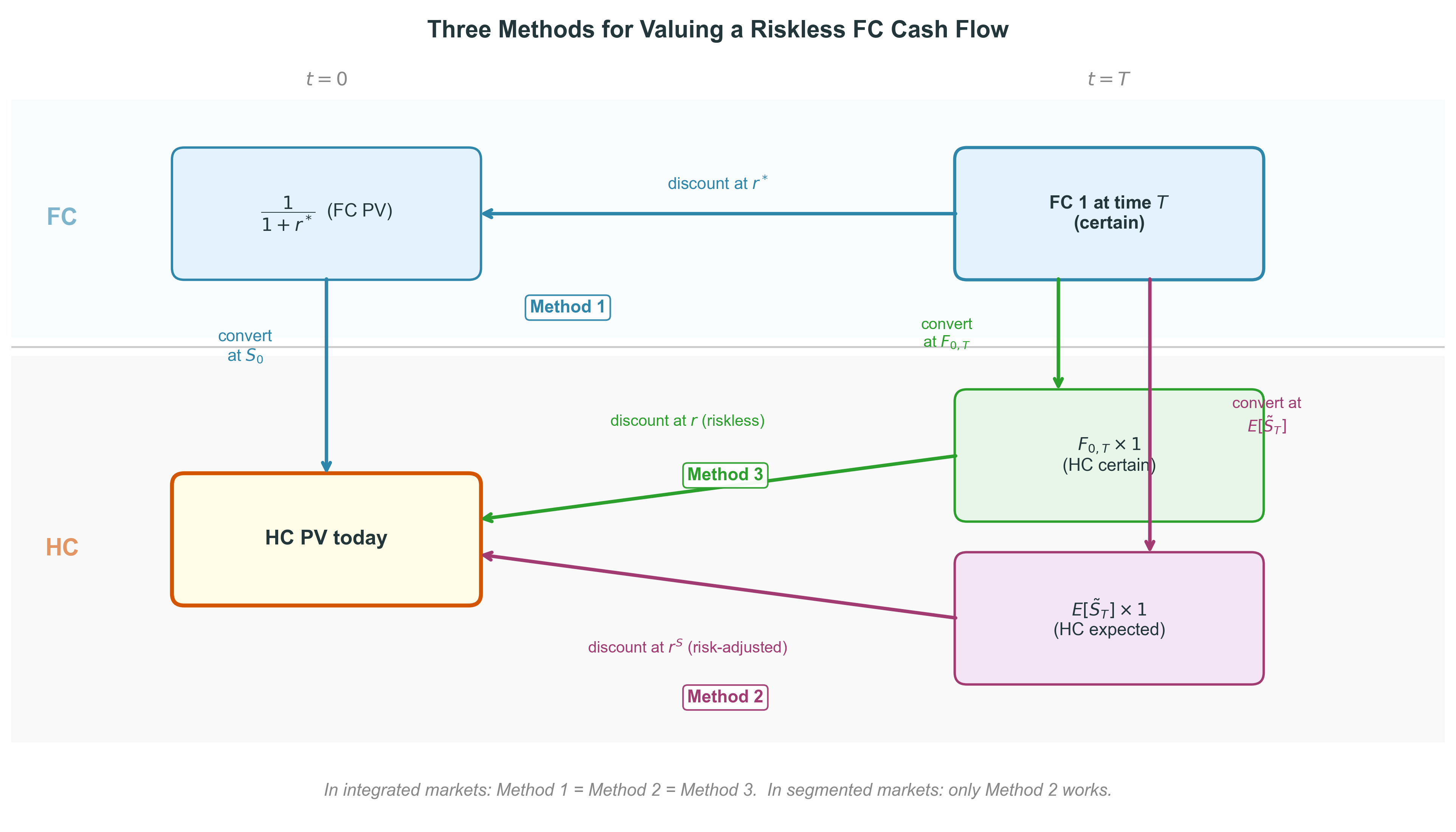
Three methods (riskless FC cash flow)

This is the “board drawing” from the video lectures, now as a figure. The three routes all start at FC 1 at time T and arrive at HC PV today, but they take different paths through the time-currency grid. Method 1 goes down first (discount), then left (convert). Method 3 goes left first (forward), then down (discount). Method 2 goes diagonally, using the expected spot rate and a risk-adjusted discount rate.

Method 1: Discount in FC, then convert

First find the present value in FC by discounting at the FC rate. Then convert the FC present value into HC by multiplying by today’s valuation spot \(S_0\) (EUR/USD).

\[PV^{HC}_0 \;=\; S_0 \times \frac{C^{FC}_T}{(1 + r^{FC})^{T}}.\]

For a unit FC cash flow:

\[PV^{HC}_0 \;=\; \frac{S_0}{(1 + r^{FC})^{T}}.\]

Logic. The FC present value is known today, so converting at today’s spot \(S_0\) is appropriate.

Method 2: Convert at expected spot, then discount

First estimate the HC value of the FC cash flow at maturity: \(\widetilde{S}_T \times C^{FC}_T\). Then discount this risky HC cash flow at a risk-adjusted HC discount rate that reflects both project risk and FX risk.

\[PV^{HC}_0 \;=\; \frac{E\!\left[\widetilde{S}_T \times C^{FC}_T\right]}{(1 + r^{HC}_{C,S})^{T}}.\]

For a unit (riskless) FC cash flow:

\[PV^{HC}_0 \;=\; \frac{E[\widetilde{S}_T]}{(1 + r^{S})^{T}}.\]

Note. This requires an explicit exchange-rate forecast and the correct FX risk adjustment — both are difficult (Lecture 5).

Method 3: Convert at forward rate, then discount

Use a forward contract to lock in today the HC value of the FC cash flow: \(F^S_{0,T} \times C^{FC}_T\). This HC value is certain, so discount it at the HC risk-free rate.

\[PV^{HC}_0 \;=\; F^S_{0,T} \times \frac{C^{FC}_T}{(1 + r^{HC})^{T}}.\]

For a unit FC cash flow:

\[PV^{HC}_0 \;=\; \frac{F^S_{0,T}}{(1 + r^{HC})^{T}}.\]

Logic. The forward eliminates FX risk; the resulting HC cash flow is riskless, so it gets the riskless discount rate. Because \(F^S\) is EUR/USD, conversion is multiplication.

Do the three methods agree?

Methods 1 and 3 are identical in integrated markets — this is just CIP rearranged. Under our valuation convention, with \(S_t\) in EUR/USD:

\[\frac{F^S_{0,T}}{S_0} \;=\; \left(\frac{1 + r^{HC}}{1 + r^{FC}}\right)^{\!T}, \qquad \text{equivalently} \qquad F^S_{0,T} \;=\; S_0 \cdot \left(\frac{1 + r^{HC}}{1 + r^{FC}}\right)^{\!T}.\]

Therefore:

\[\frac{S_0}{(1 + r^{FC})^{T}} \;=\; \frac{F^S_{0,T}}{(1 + r^{HC})^{T}}.\]

Methods 2 and 3 are identical if the HC discount rate \(r^{HC}_{C,S}\) correctly incorporates the FX risk premium. The forward rate is the certainty equivalent of the future spot (Lecture 4).

In integrated financial markets: Method 1 \(=\) Method 2 \(=\) Method 3.

Optional: in market-quote form (with \(X_t\) in USD/EUR) the same CIP relation reads \(F^X_{0,T}/X_0 = ((1+r^{USD})/(1+r^{EUR}))^{T}\). The valuation form above is what we use throughout.

EuroCorp: riskless cash-flow example

EuroCorp will receive a certain USD 5M in one year. Recall \(S_0 = 0.9091\) EUR/USD and \(F^S_{0,1} = 0.8961\) EUR/USD.

Method 1. Discount in USD, then multiply by \(S_0\).

\[PV^{USD}_0 \;=\; \frac{5}{1.045} \;=\; \text{USD } 4.785\text{M.}\] \[PV^{EUR}_0 \;=\; 0.9091 \times 4.785 \;=\; \text{EUR } 4.350\text{M.}\]

Method 3. Lock in EUR at the forward, then discount at the EUR rate.

\[\text{Locked EUR CF at } t = 1 \;=\; 5 \times 0.8961 \;=\; \text{EUR } 4.480\text{M.}\] \[PV^{EUR}_0 \;=\; \frac{4.480}{1.030} \;=\; \text{EUR } 4.350\text{M.} \quad\checkmark\]

Both methods give EUR 4.350M. CIP guarantees this. (Equivalent to dividing by the market quotes \(X_0\) and \(F^X_{0,1}\).)

We use multiplication by S and F^S as the main formula because S is EUR/USD by convention; the equivalent division by X = USD/EUR is only a sanity check.

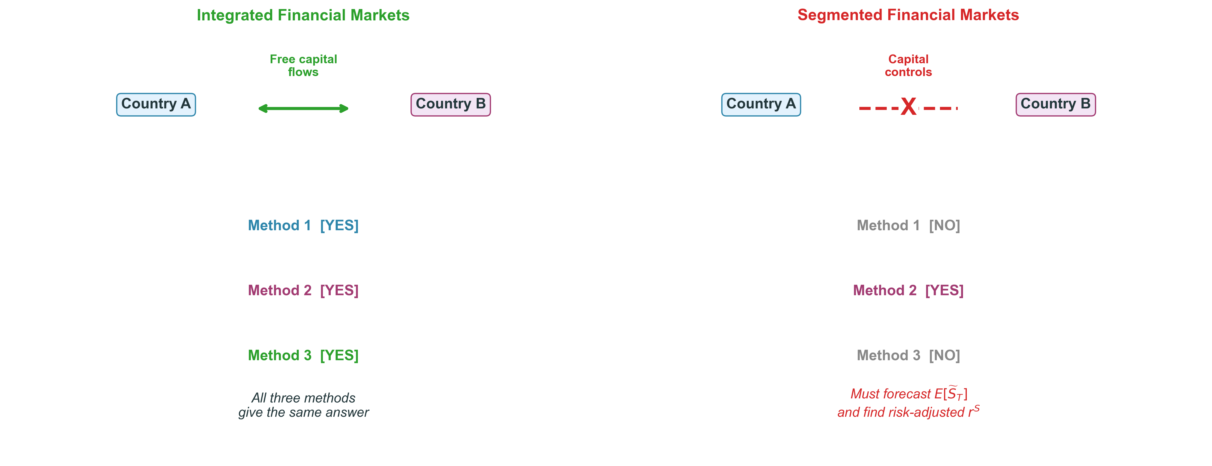
What if markets are segmented?

Segmented markets: only Method 2 works

If financial markets are segmented (capital controls, restricted forward access):

• Method 1 fails: No mechanism equates HC value and translated FC value

  • Investors in each country may discount differently — no arbitrage links them

• Method 3 fails: No liquid forward market; CIP doesn’t hold

  • Can’t lock in a forward rate if the market doesn’t exist

• Only Method 2 works. For a real project: forecast \(E[\widetilde{S}_T \times \widetilde{C}^{FC}_T]\) and discount at the appropriate HC risk-adjusted rate \(r^{HC}_{\text{proj},S}\). (For the unit riskless example: forecast \(E[\widetilde{S}_T]\) and use \(r^S\).)

This is bad news — exchange-rate forecasts are unreliable (Lecture 5: random walk).

Practical rule. In integrated markets (EUR/USD, GBP/USD, JPY/USD): use Method 3 for riskless cash flows or Method 1 for risky project cash flows. In EM with capital controls: you may be forced into Method 2.

Risky FC cash flows: Method 1

Now the FC cash flow itself is uncertain: \(\widetilde{C}^{FC}_T\).

Method 1 — Discount in FC, then convert.

\[PV^{HC}_0 \;=\; S_0 \times \frac{E[\widetilde{C}^{FC}_T]}{(1 + r^{FC}_{\text{proj}})^{T}}\]

where \(r^{FC}_{\text{proj}}\) is the risk-adjusted FC discount rate for the project.

Symbols: \(S_T\) is EUR/USD; \(\widetilde{C}^{FC}_T\) is the USD cash flow; \(S_T \times \widetilde{C}^{FC}_T\) is the EUR cash flow.

Risky FC cash flows: Method 2

Method 2 — Convert, then discount.

\[PV^{HC}_0 \;=\; \frac{E\!\left[\widetilde{S}_T \times \widetilde{C}^{FC}_T\right]}{(1 + r^{HC}_{\text{proj},S})^{T}}\]

where \(r^{HC}_{\text{proj},S}\) reflects both project risk and FX risk. The numerator is the expected EUR cash flow at maturity; discounting at \(r^{HC}_{\text{proj},S}\) gives the EUR present value today.

The covariance complication

In Method 2 the numerator is \(E[\widetilde{S}_T \times \widetilde{C}^{FC}_T]\). In general,

\[E\!\left[\widetilde{S}_T \times \widetilde{C}^{FC}_T\right] \;\neq\; E[\widetilde{S}_T] \times E[\widetilde{C}^{FC}_T]\]

unless \(\widetilde{S}_T\) and \(\widetilde{C}^{FC}_T\) are independent. In practice they are often correlated (e.g., when USD weakens against EUR, \(S_T\) falls and EUR-translated USD revenues fall; commodity exporters: FC revenues and FX often move together).

Implication. You cannot simply multiply an FX forecast by a CF forecast — you must account for the covariance, or use Method 1 in integrated markets.

This is why Method 1 is often preferred in practice for integrated markets: you can forecast CFs in FC (the currency they’re naturally generated in), discount at the FC rate, and convert at spot. You never need an FX forecast, and the covariance issue disappears. Method 2 is more general but requires more inputs and is trickier to implement correctly.

Risky CFs: equivalence in integrated markets

Methods 1 and 2 give the same answer if the discount rates are consistent. Conceptually:

\[r^{HC}_{\text{proj},S} \;\approx\; r^{FC}_{\text{proj}} \;+\; \text{expected change in } S \;+\; \text{covariance adjustment.}\]

An intuition, not a mechanical rule.

With \(S_t\) in EUR/USD: \(S_t \uparrow\) means USD appreciates vs EUR; \(S_t \downarrow\) means USD depreciates.

Practical rule. In integrated markets (US, EU, UK, JP), use Method 1: forecast CFs in their natural currency, discount at the local project rate, then multiply by \(S_0\).

WACC for Cross-Border Projects

WACC recap

\[r_{WACC} \;=\; \frac{D}{V} \cdot r_D \cdot (1 - \tau) \;+\; \frac{E}{V} \cdot r_E.\]

Simplifying assumptions:

• Market risk of project \(=\) average market risk of the firm.
• Debt-to-equity ratio is constant.
• Corporate taxes are the only market imperfection.

Levered project value:

\[V^L \;=\; \sum_{t=1}^{T} \frac{E[\text{FCF}_t]}{(1 + r_{WACC})^{t}}.\]

Compact and familiar — one discount rate captures everything.

What changes internationally?

Cost of equity \(r_E\):

• Which market portfolio? Domestic index or global index?
• Does FX risk carry a separate premium? (ICAPM lecture)

Cost of debt \(r_D\):

• Currency-specific: USD debt vs. EUR debt have different rates
• Basis-adjusted: synthetic funding cost \(\neq\) direct cost (Lecture 9)

What changes internationally? (cont.)

Tax shield:

• Which country’s tax rate? Parent’s or subsidiary’s?
• For EuroCorp: Germany (\(\tau = 30\%\)) vs. the US (\(\tau = 21\%\)). Depends on where the debt sits.

Leverage ratio:

• Measured in which currency? Market values fluctuate with FX.
• FX changes the measured leverage when debt and project value are in different currencies, or when parent-level leverage is measured on consolidated value. Pure unit conversion alone does not change \(D/V\).

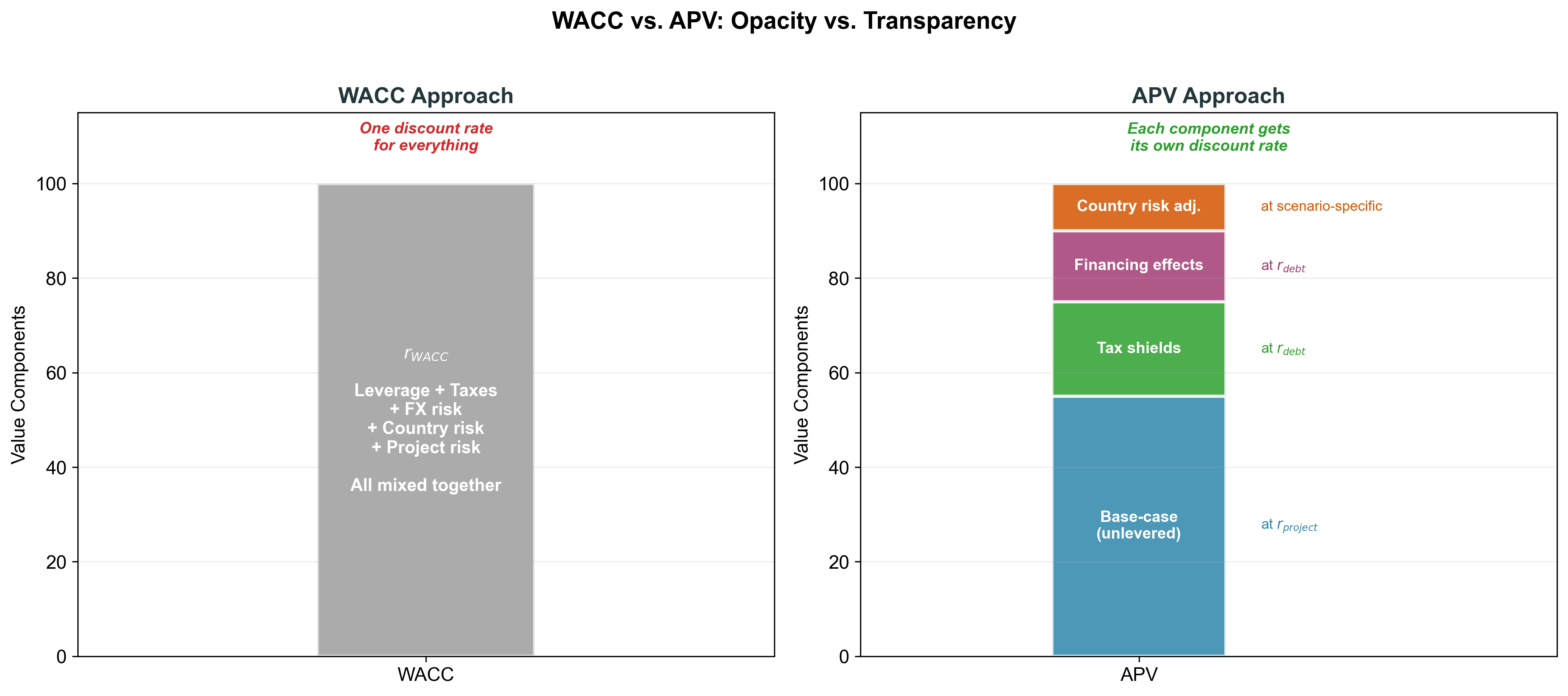
WACC limitations for international projects

1. Opaque: Mixes leverage, taxes, FX, and country risk into one number — can’t see where value comes from

2. Constant leverage: Hard to maintain when FX moves change relative values of assets and debt

3. Country risk: Where does it go? “Add 500bp to WACC” is the most common and worst practitioner approach

4. Circularity: Need market value weights to compute WACC, but need WACC to compute market values

The “500bp fallacy” is the single most important practical error this lecture needs to correct. When practitioners face country risk, they often just add a spread to the WACC. This is wrong because: (1) it double-counts risks already in the cash flows; (2) it doesn’t distinguish systematic from idiosyncratic risk; (3) it compounds over time, becoming absurdly large for long-horizon projects. We introduce it here and demolish it fully in the country risk lecture.

EuroCorp: WACC valuation

Parameters: \(r_D^{USD} = 5.5\%\), \(r_E^{USD} = 12\%\), \(\tau_{US} = 21\%\), \(D/V = 40\%\)

\[r_{WACC} = 0.40 \times 5.5\% \times (1 - 0.21) + 0.60 \times 12\% = 8.94\%\]

USD project value:

\[V^L = \sum_{t=1}^{10} \frac{9\text{M}}{(1.0894)^t} = 9\text{M} \times \frac{1 - (1.0894)^{-10}}{0.0894} = \text{USD } 57.9\text{M}\]

NPV in USD: \(57.9 - 55.0 = \text{USD } 2.9\text{M}\)

NPV in EUR: \(2.9 \times 0.9091 = \text{EUR } 2.7\text{M}\) (equivalent to dividing by the market quote \(X_0 = 1.10\) USD/EUR).

The project creates value. But where does the value come from? WACC doesn’t tell us.

This is a clean WACC calculation. Students should be comfortable with the mechanics. The point is not that WACC is wrong — it gives the right answer under its assumptions — but that it’s opaque. We don’t know how much of the USD 58.2M comes from operating cash flows vs. tax shields vs. financing effects. APV will decompose this.

APV for International Projects

APV: the logic

Start from the same place as Lecture 6 (hedging) and Lecture 9 (financing): Modigliani-Miller.

In a frictionless world: \(V^L = V^{UL}\) (capital structure irrelevant)

With frictions (taxes, subsidies, country risk):

\[V^{APV} = V^{UL} + PV(\text{financing side effects}) + \text{country risk adjustment}\]

Key advantage: Each component is separately identified, discounted at its own appropriate rate, and transparent about where value comes from.

WACC vs. APV: opacity vs. transparency

The five-step international APV

Step 1: Branch stage — operating cash flows

Treat the foreign subsidiary as an unincorporated branch of the parent.

• Focus on pure economics: revenues, costs, capex, working capital

• Ignore all financial arrangements (no debt, no intercompany transfers)

• This is the project’s value on its own merits

Discount rate: Unlevered cost of equity (project’s systematic risk only).

\[V^{UL} = \sum_{t=1}^{T} \frac{E[\text{FCF}_t]}{(1 + r_{project})^t}\]

Open question: What is \(r_{project}\)? This is answered by the ICAPM (next lecture).

Why “branch stage”? Because we’re asking: if this subsidiary were just a department of the parent with no separate legal identity, what would it be worth? This isolates the operational economics from all the financial engineering. It’s the most important number — if the branch stage NPV is negative, no amount of tax planning will save the project.

Step 2: Internal financing adjustments

Now the subsidiary is a separate legal entity.

Analyze intra-company financial arrangements:

• Dividend policy: When and how much does the subsidiary remit?

• Royalties and management fees: Payments for IP or services

• Transfer pricing: Prices on intra-firm goods/services

• Intercompany loans: Parent lending to subsidiary (or vice versa)

These affect taxes, FX exposure, and political risk.

Practical caveat: Tax planning is complex, evolving, and risky. Safer to accept projects primarily on their economic merits (Step 1).

Discount rate: Appropriate rate for each flow (often close to risk-free if contractual).

Step 3: External financing adjustments

The value created (or destroyed) by the firm’s financing choices:

• Tax shields from debt: PV of interest tax deductions
  • Who borrows? Parent (Germany) or subsidiary (US)?
  • Tax shield = \(\tau \times r_D \times D\) per year (if debt is constant)
• Where to borrow, in what currency? Connects to Lecture 9
  • Basis-adjusted funding cost; natural hedging benefits
• Subsidized financing: Export credit agencies, development bank loans

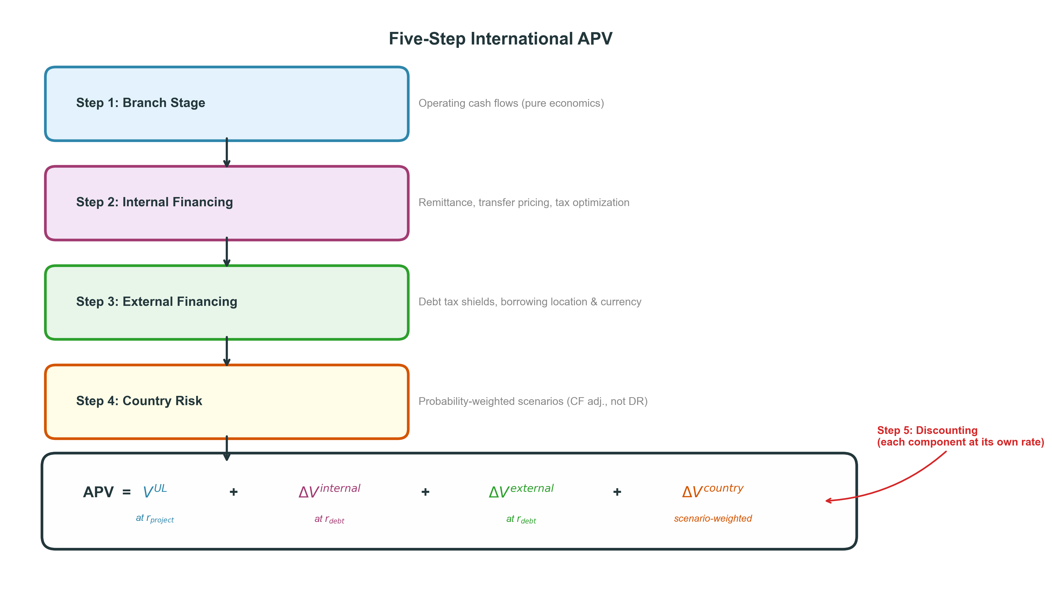
Discount rate. For a fixed debt schedule, tax shields are usually discounted at the cost of debt, because the shield inherits the debt’s risk. With target leverage, the debt grows with project value and the tax-shield risk is closer to project risk; many practitioners then discount at the unlevered cost of equity.

PV of tax shields under a fixed debt schedule

\[PV(\text{tax shields}) \;=\; \sum_{t=1}^{T} \frac{\tau \times r_D \times D_t}{(1 + r_D)^{t}}.\]

For a fixed debt schedule, the tax shield is tied to promised interest payments of known size — that is why practitioners often discount it at \(r_D\). With target leverage, the debt moves with project value, so the tax shield’s risk is closer to project risk and the discount rate moves toward the unlevered cost of equity.

Step 4: Country risk adjustments

Preview only — full treatment in the Country Risk lecture.

Key principle: model idiosyncratic political/country scenarios in the cash flows; keep systematic risk in the discount rate.

• Enumerate scenarios (base case, tariff, sanctions, expropriation).
• Assign probabilities to each scenario.
• Expected CF \(=\) probability-weighted average.

More transparent than “add 500 bp to WACC” because:

• Each scenario is explicit and auditable.
• Idiosyncratic risks enter the cash flows (probability haircut), not the discount rate.
• Only systematic risk enters the discount rate.

For EuroCorp’s US project: country risk is minimal — but would be critical for an EM project.

Step 5: Discounting

Different discount rates for different components:

Component	Discount Rate	Rationale
Operating CFs (Step 1)	Unlevered cost of equity	Project’s systematic risk
Internal financing (Step 2)	Near risk-free	Contractual flows
Tax shields (Step 3)	Cost of debt	Debt-like risk
Country risk (Step 4)	Scenario-specific	Depends on risk type

This is why APV is superior: each cash flow stream gets the rate that matches its risk.

WACC forces all components through a single rate — which can only be “right” for the average flow, not for any individual one.

EuroCorp: APV valuation

Step 1: Unlevered value (at \(r_{project} = 10\%\))

\[V^{UL} = \sum_{t=1}^{10} \frac{9\text{M}}{(1.10)^t} = 9\text{M} \times 6.1446 = \text{USD } 55.3\text{M}\]

Step 3: Tax shields (US debt \(\approx\) USD 22M, \(\tau = 21\%\), \(r_D = 5.5\%\))

\[\text{Annual TS} = 0.21 \times 0.055 \times 22\text{M} = \text{USD } 0.254\text{M} \quad \Rightarrow \quad PV = \text{USD } 1.91\text{M}\]

Steps 2, 4: Minimal for this US project (no complex transfer pricing; low country risk).

\[V^{APV} \;=\; 55.3 + 1.91 \;=\; \text{USD } 57.2\text{M,} \qquad \text{NPV} \;=\; 57.2 - 55.0 \;=\; \text{USD } 2.2\text{M.}\]

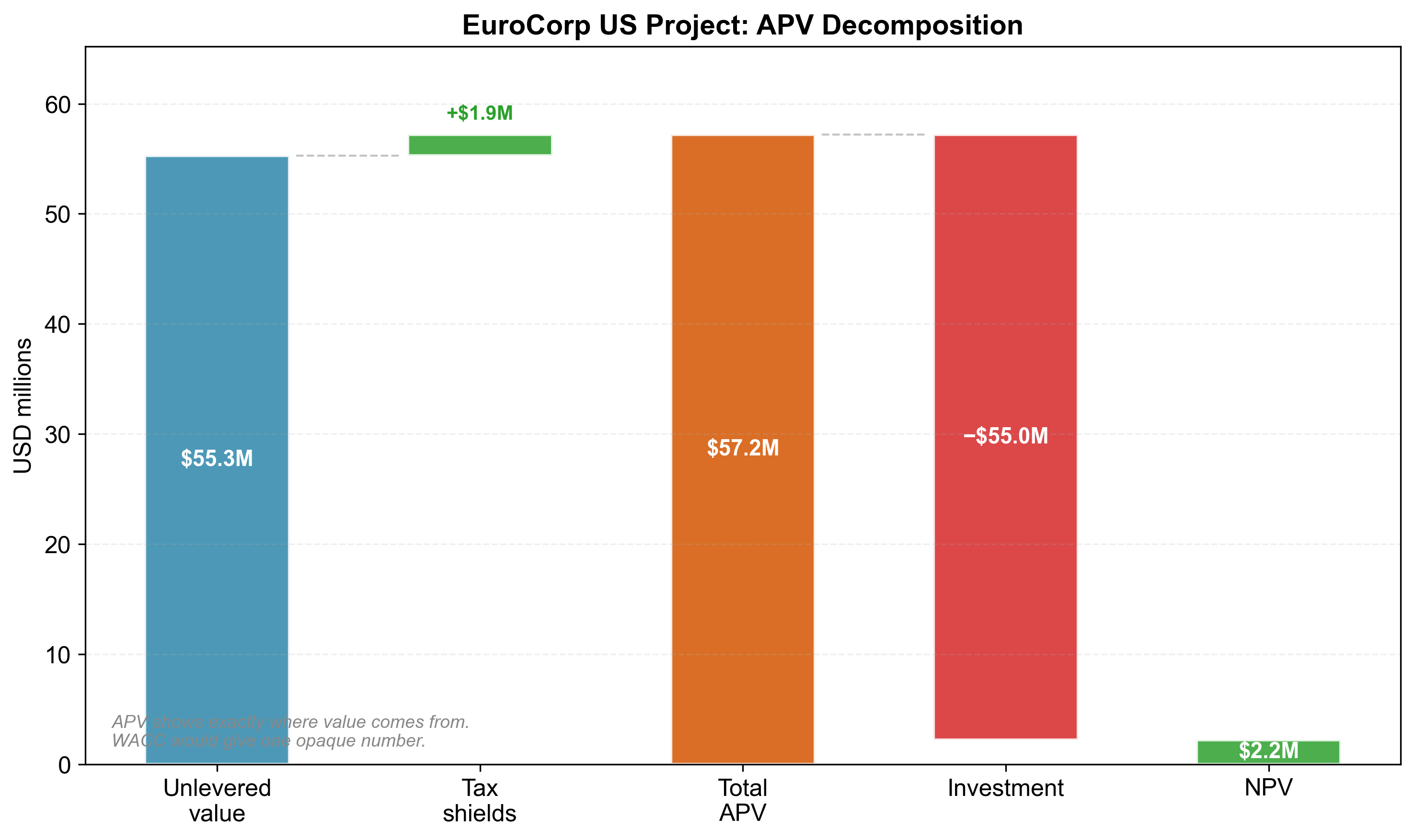
Why does this differ from the WACC NPV (USD 2.9M)? The WACC example assumes a constant target \(D/V\) ratio of 40%, so the implicit tax-shield value grows with project value. This APV example uses a fixed USD 22M debt schedule. WACC and APV give the same value only when the leverage and risk assumptions are aligned.

APV decomposition

The waterfall chart makes APV’s advantage concrete. We can see exactly how much of the project’s value comes from operating cash flows (USD 55.3M) vs. tax shields (USD 1.9M). After subtracting the USD 55M investment, the NPV is USD 2.2M. If we were to add country risk (e.g., for a Brazilian project), it would appear as a separate negative bar — making the cost explicit and auditable. WACC would hide all of this in a single blended rate.

APV vs. WACC: the comparison

Feature	WACC	APV
Simplicity	One rate, one DCF	Multiple components
Transparency	Low — all mixed	High — each part visible
Constant leverage?	Required	Not needed
Country risk	“Add 500 bp” (bad)	Explicit CF adjustment (good)
Financing effects	Embedded in rate	Separated and valued
When to use	Quick domestic check	Cross-border projects

WACC and APV give the same answer when leverage is truly constant, country risk is absent, and project risk equals firm-average risk. For international projects these rarely all hold — use APV.

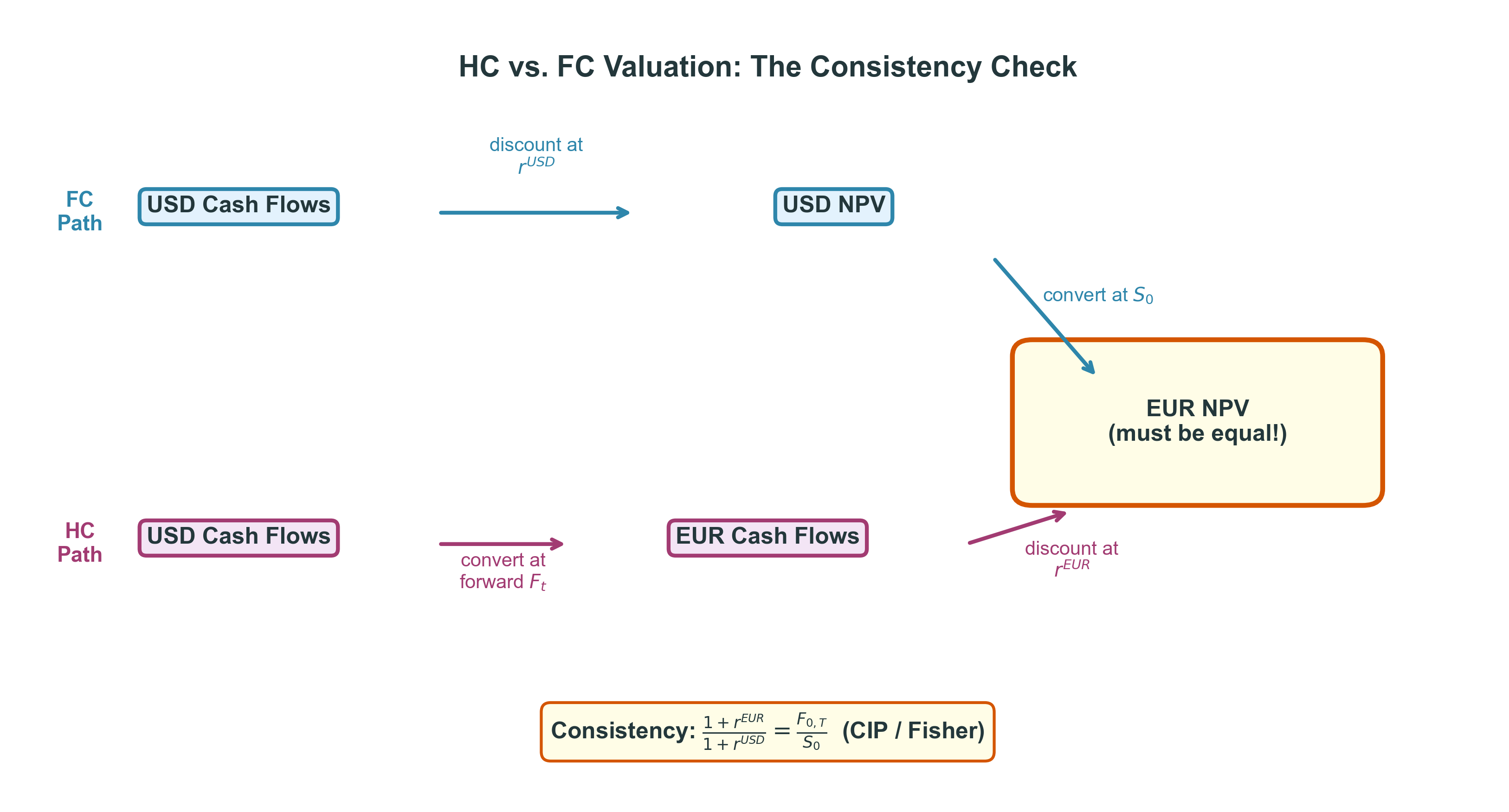
HC vs. FC Valuation: The Consistency Check

Two equivalent DCF approaches

You can value EuroCorp’s US project in either currency.

FC approach (USD).

1. Forecast project cash flows in USD.
2. Discount at the USD project discount rate.
3. Multiply by \(S_0 = 0.9091\) EUR/USD to convert the USD value to EUR.

HC approach (EUR).

1. Multiply each USD cash flow by the EUR/USD forward \(F^S_{0,t}\) to get EUR cash flows.
2. Discount those EUR cash flows at the EUR-consistent project discount rate.
3. The result must match the FC approach.

Both must give the same EUR NPV.

The consistency condition

Why must they agree?

CIP, in valuation form (with \(S_t\) in EUR/USD and \(F^S_{0,t}\) the EUR/USD forward):

\[\frac{F^S_{0,T}}{S_0} \;=\; \left(\frac{1 + r^{EUR}_{rf}}{1 + r^{USD}_{rf}}\right)^{\!T}, \qquad \text{i.e.} \qquad F^S_{0,t} \;=\; S_0 \times \left(\frac{1 + r^{EUR}_{rf}}{1 + r^{USD}_{rf}}\right)^{\!t}.\]

The EUR project discount rate consistent with the USD project discount rate is:

\[1 + r^{EUR}_{\text{proj}} \;=\; \bigl(1 + r^{USD}_{\text{proj}}\bigr) \times \frac{1 + r^{EUR}_{rf}}{1 + r^{USD}_{rf}}.\]

The risk-free interest differential adjusts the currency of the discount rate; it is not an extra project-risk premium.

If you use USD CFs with USD rates, or EUR CFs (converted via \(F^S\)) with EUR rates, the present values are identical.

Common errors that break consistency

1. Mixing quote conventions: using the market quote \(X_t\) (USD/EUR) in formulas that require the valuation rate \(S_t\) (EUR/USD).
2. Dividing by \(S\) when \(S\) is already EUR/USD — conversion should be multiplication.
3. Currency–rate mismatch: discounting USD cash flows at an EUR rate (or vice versa) mixes numeraires.
4. Inconsistent forward or forecast that contradicts the interest-rate differential implied by CIP.
5. Double-counting FX risk in both cash flows and the discount rate.
6. Confusing rates and discount factors: the “1.10” in the Year-1 USD path is the project discount factor, not the exchange rate.

Each of these makes the FC and HC paths disagree — and the size of the disagreement scales with horizon.

EuroCorp consistency check: USD path

A Year-1 cash flow of USD 9M, USD project rate \(10\%\), \(S_0 = 0.9091\) EUR/USD.

Discount in USD, then multiply by \(S_0\):

\[PV^{USD}_0 \;=\; \frac{9}{1.10} \;=\; \text{USD } 8.182\text{M.}\]

Here \(1.10\) is the USD project discount factor, not the exchange rate.

\[PV^{EUR}_0 \;=\; 8.182 \times 0.9091 \;=\; \text{EUR } 7.438\text{M.}\]

EuroCorp consistency check: EUR path

A Year-1 cash flow of USD 9M, \(F^S_{0,1} = 0.8961\) EUR/USD.

Forward-converted EUR cash flow:

\[CF^{EUR}_1 \;=\; 9 \times 0.8961 \;=\; \text{EUR } 8.065\text{M.}\]

EUR project discount rate from the rate differential:

\[1 + r^{EUR}_{\text{proj}} \;=\; (1 + r^{USD}_{\text{proj}}) \times \frac{1 + r^{EUR}_{rf}}{1 + r^{USD}_{rf}} \;=\; 1.10 \times \frac{1.030}{1.045} \;=\; 1.0842, \;\;\Rightarrow\;\; r^{EUR}_{\text{proj}} \approx 8.42\%.\]

\[PV^{EUR}_0 \;=\; \frac{8.065}{1.0842} \;=\; \text{EUR } 7.438\text{M.} \quad\checkmark\]

Both paths give the same EUR 7.438M.

PV_0 not PV_1 — both are present values today (at t=0) of a Year-1 cash flow. The exact EUR project rate is 8.42%; that makes the two paths agree to three decimals.

Practical guidance

Which approach to use?

• FC approach (discount in USD) is usually simpler:

  • Cash flows are naturally generated in USD

  • No need to forecast exchange rates

  • Just discount at the USD project rate and convert once at spot

• HC approach (convert via forwards) is useful when:

  • Management wants to see EUR cash flows

  • Comparing projects across multiple foreign currencies

  • Building consolidated EUR-denominated financial plans

• Always check consistency: if the two approaches give different answers, there is an error in your assumptions.

Caveats for Cross-Border Valuation

Practical warnings

1. Don’t use speculative currency forecasts. Use forward rates whenever possible.

   • If forwards aren’t available, check that your forecast is within the range implied by the interest rate differential.

2. Be careful comparing multiples across countries. P/E ratios differ due to accounting standards, growth rates, and risk premia — not just “cheapness.”

3. Market risk premium: Take the perspective of the actual shareholders who will bear the risk. If the firm’s shareholders are globally diversified, use the global market premium.

4. Sensitivity analysis: Difficult-to-quantify aspects (country risk, regulatory change, competitive response) make cross-border valuations inherently uncertain. After finding the APV, stress-test your assumptions.

Summary and Connections

Key takeaways

1. Three methods for valuing FC cash flows: Discount-then-convert, convert-then-discount, forward-then-discount. All equivalent in integrated markets; only Method 2 in segmented markets.

2. WACC works but is opaque. It mixes leverage, taxes, FX, and country risk into one rate. Fine for a quick domestic check; dangerous for cross-border projects.

3. APV is the preferred framework. Five-step approach separates operating value, internal/external financing, and country risk. Each component gets its own discount rate.

4. Consistency check: HC and FC approaches must give the same answer. If they don’t, there’s an error.

5. Open question: What discount rate for the base case? \(\to\) answered in the ICAPM lecture.

Connections to the course

• Lecture 4 (CIP): CIP guarantees Methods 1 and 3 are equivalent. Without CIP, Method 3 fails.

• Lecture 5 (UIP/Predictability): Exchange rate forecasts are unreliable — use forward rates, not speculative forecasts (Method 3 over Method 2 when possible).

• Lecture 6 (Why Hedge?): MM logic underpins APV. Frictionless \(\to\) irrelevant; frictions \(\to\) APV adjustments.

• Lecture 9 (Financing): Where and how to borrow feeds directly into APV Step 3. The basis affects the cost of financing.

• Next lecture (ICAPM): Answers “what is \(r_{project}\)?” — the discount rate for APV Step 1.

• Country Risk lecture: Answers “how does country risk enter?” — APV Step 4 in detail.

The course architecture is now clear: this lecture builds the APV framework (the “where to put things”). The ICAPM lecture fills in the discount rate (the “what rate”). The country risk lecture fills in the CF adjustments (the “how to adjust”). Together, these three lectures complete the investment decision.